Download
1 / 30
300 likes | 321 Views
Explore annual temperature and precipitation patterns in North, Central, and South America from various meteorological sources. Understand deviations from climatic norms over decades for a holistic view of regional climate trends.

E N D
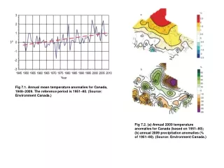
Fig 7.1. Annual mean temperature anomalies for Canada, 1948–2009. The reference period is 1951–80. (Source: Environment Canada.) Fig 7.2. (a) Annual 2009 temperature anomalies for Canada (based on 1951–80); (b) annual 2009 precipitation anomalies (% of 1951–80). (Source: Environment Canada.)
Fig. 7.3. Annual mean temperature for the contiguous United States, 1895–2009. (Source: NOAA/NCDC.) Fig. 7.4. Statewide ranks of (a) 2009 temperatures and (b) 2009 precipitation. A rank of 115 represents the warmest/wettest year since 1895. Much above-normal temperature/precipitation is defined as occurring in the top 10% of recorded years, which corresponds to a rank of 105–115. Above-normal temperature/precipitation is defined as occurring in the warmest/wettest third of recorded years (ranks 78–103). Much below-normal temperature/precipitation is likewise the bottom 10% of coolest/driest years since 1895, and below normal is defined as the remaining coolest/driest third of the distribution. (Source: NOAA/NCDC.)
Fig. 7.5. Seasonally averaged surface temperature departures (relative to 1971–2000) during 2009 based on NCDC climate division data (left panels), and climate simulations forced with observed monthly varying global sea surface temperature and sea ice conditions during 2009 (right panels). The simulations consist of 6 different models and a total ensemble size of 260 members conducted for 2009. (Source: NOAA/ESRL.) Fig 7.6. (a) Annual 2009 temperature anomalies for Mexico (based on 1971–2000); (b) annual 2009 precipitation anomalies (% of 1971–2000). (Source: National Meteorological Service of México.)
Fig. 7.7. Central America showing the location of selected stations: 1. Phillip Goldson Int. Airport, Belize; 2. Puerto Lempira, Honduras; 3. Puerto Limon, Costa Rica; 4. David, Panama; 5. Liberia, Costa Rica; 6. Choluteca, Honduras; and 7. San Jose, Guatemala. For each station, surface temperature frequency is shown on the left and accumulated pentad precipitation on the right. Blue represents climatology for the base period 1971–2000, red the 2000–09 decade and green 2009. Note that San Jose does not show 2009 precipitation data due to large amount of missing data. (Source: NOAA/NCDC.)
Fig 7.9. Monthly Jamaican rainfall for 2009 (bars), climatology (black), and one standard deviation from climatology (dashed). The reference period is 1961–90. (Source: Meteorological Service of Jamaica.) Fig. 7.8. (a) Annual mean temperature for Cuba, 1951–2009 and (b) annual precipitation anomalies, represented as Standardized Precipitation Indes, based on 1971–2000. (Source: Institute of Meteorology of Cuba.)
Fig. 7.10. Weekly mean rainfall for Puerco Rico, based on over 50 cooperative weather stations, with accumulative rainfall displayed on the right hand axis of chart. Year to date surpluses and deficits displayed with blue and red shading respectively.(Source: NOAA/NWS. Fig. 7.11. (a) Annual 2009 temperature anomalies for South America (°C; based on 1971–2000) and (b) annual 2009 precipitation anomalies (% relative to 1971–2000). Sources: National Meteorological Services of Argentina, Brazil, Bolivia, Chile, Colombia, Ecuador, Paraguay, Peru, Uruguay and Venezuela. Data compilation and processing by CIIFEN 2009.
Fig. 7.12. (a) December 2008 to February 2009 rainfall anomalies and (b) February to May 2009 rainfall anomalies (% relative to 1961–90). (Source: CPTEC/INPE.) Fig. 7.13. Monthly mean water level of the Rio Negro in Manaus, Brazil, for some extreme years: dry (1964, 2005), wet (1953, 2009), compared to the 1903–86 average. (Source: CPTEC/INPE.)
Fig. 7.14. Composite for standardized mean anomaly of daily maximum temperature along the subtropical west side of South America (Central Chile) for January- March, based on measurements at Santiago (33.5ºS), Curicó (35.0ºS) and Chillán (36.6ºS). Standardization was done using 1971–2000. (Source: Dirección Meteorológica de Chile.) Fig. 7.15. November 2009 rainfall (mm) in Southeastern South America. (Source: CPTEC/INPE.)
Fig. 7.17. Daily maximum temperature anomalies on July 21st 2009 for northwest Africa (°C; based on 1968–96). (Source: NOAA/CDC.) Fig. 7.16. November mean rainfall for Southeastern South America, 1979–2009. (Source: GPCP.)
Fig. 7.18. Annual mean temperature anomalies (based on 1961–90) for Egypt, 1975–2009. (Source: Egyptian Meteorological Authority.) Fig. 7.19. Monthly mean temperature in 2009 and 1961–90 average for Bilma, Niger. (Source: African Centre of Meteorological Applications for Development.)
Fig. 7.20. (a) July to September 2009 rainfall (mm) for Western and Central Africa and (b) July to September 2009 anomalies (expressed as percentage of 1971–2000.) (Source: NOAA/NCEP.) Fig. 7.21. (a) December 2008 to February 2009 rainfall anomalies and (b) October to December 2009 rainfall anomalies (expressed as percentage of 1961–90) for the Great Horn of Africa. (Source: ICPAC, 2009.)
Fig. 7.23. Annual mean temperature anomalies (based on 1961–90) average over 27 stations in South Africa, 1961–2009. (Source: South African Weather Service.) Fig. 7.22. Cumulative rainfall for (a) Neghelle, Ethiopia, (b) Dagoretti, Kenya and (c) Kigoma, Tanzania. (Source: ICPAC, 2009.)
Fig. 7.24. Rainfall 2009 anomalies (expressed as percentage of 1961–90) for South Africa for 2009. (Source: South African Weather Service.) Fig. 7.25. (a) December 2008 to February 2009 rainfall (mm) for Southern Africa and (b) December 2008 to February 2009 anomalies (expressed as percentage of 1971–2000). (Source: NOAA/NCEP.)
Fig. 7.27. (a) Annual 2009 temperature anomalies (°C; based on 1971–2000) and (b) annual 2009 precipitation anomalies (% of 1971–90) for Madagascar. (Source: Service Météorologique de Madagascar.) Fig. 7.26. (a) Annual 2009 temperature anomalies (°C; based on 1971–2000) and (b) annual 2009 precipitation anomalies (% of 1971–2000) for the countries of the Western Indian Ocean. (Source: Météo Nationale Comorienne, Service Météorologique de Madagascar, Météo-France, Mauritius Meteorological Services and Seychelles National Meteorological Services.)
Fig. 7.28. Annual mean temperature anomalies for La Reunion (average of 10 stations observations), 1970–2009. (Source: Météo-France.) Fig. 7.29. Annual mean anomalies of surface air temperature in Europe and over the North Atlantic, 2009 (°C, 1961–90 base period), CRUTEM3 data updated from Brohan et al. 2006. (Source: UK Met Office.)
Fig. 7.30. European precipitation totals (% of normal, 1951–2000 base) for 2009. (Source: Global Precipitation Climatology Centre [GPCC], Rudolf et al. 2005.) Fig. 7.31. Seasonal anomalies (1961–90 reference) of 500 hPa geopotential height (contour, gpm) and 850 hPa temperature (shading, K) using data from the NCEP/NCAR reanalysis. (DJF) winter (Dec 2008–Feb 2009), (MAM) spring (Mar–May 2009), (JJA) summer (Jun–Aug 2009) and (SON) autumn (Sep–Nov 2009). Black (white) thick lines highlight those geopotential height (temperature) contours with all the encircled grid points having absolute anomalies above their 1-sigma level of the base period.
Fig. 7.32. European land surface air temperature anomalies (°C, 1961–90 base period), CRUTEM3 updated from Brohan et al. 2006. (a) December 2008 to February 2009; (b) March to May 2009; (c) June to August 2009; (d) September to November 2009. Fig. 7.33. Seasonal anomalies, with respect to the 1961-90 mean, of sea level pressure (hPa) from NCAR/NCEP reanalyses. Colored shading represents the percentage of accumulated seasonal precipitation compared with the 1951–2000 climatology from the seasonal GPCC precipitation data set (only values above 15 mm per season are represented). Thick black lines highlight those sea level pressure anomalies which are greater than one standard deviation above the mean.
Fig. 7.34.Monthly mean anomalies of surface air temperature across Europe and over the North Atlantic, April 2009 (°C, 1961–90 base period) based on CLIMAT and ship observations. [Source: Deutscher Wetterdienst (DWD).] Fig. 7.35. Rainfall across northwest England from 0900 UTC on 17th to 0900 on 20th November 2009.
Fig. 7.37. Anomalies of annual mean air temperature averaged over the Russian territory for the period 1939–2009 (base period: 1961–90). Fig. 7.36. Maximum wind gusts recorded in Spain and southern France (on either 23 or 24 January 2009). Green (100–120 km/h), yellow (120–140 km/h), orange (140–160 km/h), red (160–180 km/h), and brown (180–200 km/h). Stations which set new wind gust records are highlighted with a solid circle around the color circle.
Fig. 7.38. Air temperature anomalies in April 2009. Insets show mean April air temperatures and mean daily air temperatures in April 2009 at meteorological stations Khabarovsk, Makhachkala and Tura; (a) Number of days with high temperature extremes in April 2009; (b) Number of days with low temperature extremes in April 2009.
Fig. 7.39. Weather conditions in December 2009 (a) Air temperature anomalies. Insets show the series of mean monthly and mean daily air temperatures in December 2009 at meteorological stations Pechora, Baikit, Markovo, and Kazan; (b) Percentage of monthly mean precipitation in the southern Far East. Insets show the series of monthly and daily precipitation totals in December 2009 at meteorological station Vladivostok.
Fig. 7.40. Annual mean temperature anomalies (°C; 1971–2000 base period) over East Asia in 2009. (Source: Japan Meteorological Agency.) Fig. 7.41. Annual precipitation ratio as percentage of normal (1971–2000 base period) over East Asia in 2009. (Source: Japan Meteorological Agency.)
Fig 7.42. Variation of pentad zonal wind index over the monitoring region (10°N–20ºN, 110°E–120ºE). Red open bars are climatology (Unit: m s–1) (Source: China Meteorological Administration.) Fig 7.43. Annual mean temperature anomalies (with respect to 1961–90 normal) averaged over India for the period 1901–2009. The smoothed time series (9-point binomial filter) is shown as a continuous line.
Fig 7.44. Monsoonal (Jun–Sep) rainfall over India in 2009. (a) actual, (b) normal (base period) and, (c) anomalies (with respect to base period.) Fig 7.45. Daily standardized rainfall time series averaged over the monsoon region of India (1 June to 30 September 2009).
Fig. 7.46. 2009 Rainfall percentage of 1949–90 normal. (Source: U.S. Air Force, 14th Weather Squadron.) Fig. 7.47. Spring mean temperature anomaly (°C; base period 1989–2008) for Iran. (Source: Islamic Republic of Iran Meteorological Organization.)
Fig. 7.49 Australian mean annual maximum temperature anomalies (base period 1961–90) for 2009. Fig. 7.48. Spring precipitation (percentage of the 1989–2008 normal) for Iran. (Source: Islamic Republic of Iran Meteorological Organization.)
Fig. 7.50. Australian mean annual minimum temperature anomalies (base period 1961–90) for 2009. Fig 7.51. Australian annual rainfall deciles (since 1900) for 2009.
Fig. 7.52. Maximum temperatures on 7 February 2009. Fig. 7.53. Annual and decadal mean temperature anomalies for New Zealand based upon a seven-station series. Base period: 1971–2000.
Fig. 7.54. Air temperature anomaly (1971–2000 base period) for the Southwest Pacific. (Source: NOAA NCEP CPC CAMS.) Fig. 7.55. Percentage of mean annual rainfall for 2009 (1979–95 base period) for the Southwest Pacific. (Source: NOAA NCEP CPC CAMS.)
Fig. 7.56. Rainfall as a percent of normal for selected Micronesian islands for January through June (solid green), July through December (hatched blue), and for January through December 2009 (solid tan). The percent of normal is determined from the NCDC 1971–2000 base period.