Download
1 / 44
440 likes | 550 Views
This lecture covers key concepts in second-order systems and block diagram reduction. Explore nature of responses, damping ratios, poles analysis, and system specifications. Learn how poles affect response types with examples and practical tips.

E N D
INC341Second Order Systems&Block Diagram Reduction Lecture 4
1st order review • Time constant = 1/a • Settling Time (Ts) = 4 เท่าของ time constant
Type of Systems • First-order Systems • Second-order Systems • Higher-order Systems
Second-order Systems ระบบที่มี 2 poles ตัวอย่างเช่นดังรูป จะพิจารณา Output ที่ได้ จากการป้อน Input เป็น unit step u(t)
Nature of response for 2nd order systems พิจารณาตามตำแหน่งของ poles (ลักษณะกราฟ) แบ่งได้เป็น 4 cases • Overdamped response: all poles on real axis • Underdamped response: complex poles on left-half plane • Undamped: complex poles on imaginary axis • Critically damped: repeated roots on real axis
Overdamped Underdamped Undamped Critically damped
การจะดูว่าอยู่ใน case ไหน ให้ดูที่ตำแหน่งของ poles เช่น เป็น underdamped
Undamped natural frequency (rad/sec) Damping ratio (unitless) General form of Second-order Systems • Natural frequency • Damping ratio
Poles สามารถหาได้เท่ากับ ดังนั้น ζ เป็นตัวกำหนดชนิดของ response ต่างๆได้
Distance from origin is natural frequency Natural Frequency x x Frequency at which system would oscillate if all damping was removed, i.e., frequency of oscillation of a series RLC circuit with the resistance shorted would be the natural frequency.
Damped Natural Frequency x Imaginary component is damped natural frequency x Frequency at which system actually oscillates
Angle Damping Ratio ζ = x/ω x ω x x
Example 4.4 จงบอกชนิดของ response ในแต่ละ system Clue: overdamped critically damped underdamped
System Specifications • Peak time, Tp: Time to reach maximum peak. • Percentage overshoot, %OS: The amount that the waveform overshoots the steady state of final value
Settling time Ts: Time required for oscillations to be bounded within 2% of steady state value Tp ทั้ง 3 อย่างนี้มีความสัมพันธ์กับ poles b %OS=b/a × 100% a
Line of Constant Decay Rate Real part of pole gives rate of decay All poles lying on the same vertical line will decay at same rate x Settling time Ts x
x x Line of Constant Frequency Imaginary part of pole gives oscillation frequency All poles lying on same horizontal line in s-plane have same oscillation frequency
Lines of constant damping Poles on radial lines extending out from origin have same damping ratio x x
Same settling time Same peak time Same % overshoot
Time constant and damped frequency • Time constant (second): หาได้จาก reciprocal of real part of dominant pole • Damped frequency of oscillation (radian): หาได้จาก imaginary part of dominant pole Note: dominant pole คือ pole ตัวที่อยู่ใกล้ imaginary axis มากที่สุด ซึ่งก็คือ pole ตัวที่มีผลต่อระบบมากที่สุดนั่นเอง
Questions Q: จงบอกชนิดของ response พร้อมทั้งหา time constant และ damped frequency ของระบบต่อไปนี้
ตำแหน่ง poles บอกอะไรบ้าง • Real part: บอกถึง settling time โดยที่ pole ตัวที่อยู่ใกล้ origin มากสุด, จะมี settling time มากสุด, จะทำให้เกิดผลตอบสนองต่อระบบช้าที่สุด เราเรียก pole ตัวนี้ว่า dominant pole ซึ่งเป็น pole ที่มีความสำคัญที่สุดในระบบ • Imaginary part: บอกถึงลักษณะการสั่นของสัญญาณตอบสนองที่จะเกิดขึ้น ซึ่งหมายถึง % overshoot และ peak time
Effect ofZero’s Position Zeros จะมีผลมากถ้ามันอยู่ใกล้ dominant poles (pole-zero cancellation) เช่น ระบบที่มี poles ที่ -1±j2.828 ถ้าเพิ่ม zero ณ ที่ต่างๆจะได้ผลตามรูป
Example Poles อยู่ที่ -3±j7 ให้หา Tp, Ts, %OS
Type of Systems • First-order Systems • Second-order Systems • Higher-order Systems
Higher-Order System จะประมาณเป็น second-order systems โดยดูจาก dominant poles Dominant poles คือ 2 poles ที่อยู่ใกล้แกนตั้งมากที่สุด Example 1 Overdamped Example 2 Underdamped
(∞) = Case III
Nise’s Proposition ถ้า poles ไกลกว่า dominant poles 5 เท่าของแกนจำนวนจริง จะถือว่าตัดทิ้งไปได้
conclusions • ในบทนี้จะศึกษา response ของระบบในช่วง transient เท่านั้น ซึ่งเน้นศึกษาแค่ 1st and 2nd order systems • Terms ต่างๆที่สำคัญๆคือ time constant, settling time (4 times of time constant), dominant pole, natural frequency, damping ratio (ส่งผลให้เกิด response แตกต่างกันออกไป) • ตำแหน่ง poles และ zeros มีผลต่อผลตอบสนองของระบบอย่างไร
Multiple Subsystems and Reduction หา specification ของระบบ แบ่งเป็นส่วนๆและวาด Block Diagram มองระบบรวมและเขียน Schematics วิเคราะห์ด้วย ทฤษฎี ลดรูป Block Diagram หา transfer function ของแต่ละ block
Box-moving Technique Move pass summing junction
Example ให้ลดรูปจนเหลือ block เดียว
Example ให้ลดรูปจนเหลือ block เดียว