Sparse Matrix Methods

1. Sparse Matrix Methods • Day 1: Overview • Day 2:Direct methods • Day 3: Iterative methods • The conjugate gradient algorithm • Parallel conjugate gradient and graph partitioning • Preconditioning methods and graph coloring • Domain decomposition and multigrid • Krylov subspace methods for other problems • Complexity of iterative and direct methods

2. SuperLU-dist: Iterative refinement to improve solution Usually 0 – 3 steps are enough • Iterate: • r = b – A*x • backerr = maxi ( ri / (|A|*|x| + |b|)i ) • if backerr < ε or backerr > lasterr/2 then stop iterating • solve L*U*dx = r • x = x + dx • lasterr = backerr • repeat

3. (Matlab demo) • iterative refinement

4. Convergence analysis of iterative refinement Let C = I – A(LU)-1 [ so A = (I – C)·(LU) ] x1 = (LU)-1b r1 = b – Ax1 = (I – A(LU)-1)b = Cb dx1 = (LU)-1 r1 = (LU)-1Cb x2 = x1+dx1 = (LU)-1(I + C)b r2 = b – Ax2 = (I – (I – C)·(I + C))b = C2b . . . In general, rk = b – Axk = Ckb Thus rk  0 if |largest eigenvalue of C| < 1.

5. Direct A = LU Iterative y’ = Ay More General Non- symmetric Symmetric positive definite More Robust More Robust Less Storage The Landscape of Sparse Ax=b Solvers D

6. Conjugate gradient iteration x0 = 0, r0 = b, p0 = r0 for k = 1, 2, 3, . . . αk = (rTk-1rk-1) / (pTk-1Apk-1) step length xk = xk-1 + αk pk-1 approx solution rk = rk-1 – αk Apk-1 residual βk = (rTk rk) / (rTk-1rk-1) improvement pk = rk + βk pk-1 search direction • One matrix-vector multiplication per iteration • Two vector dot products per iteration • Four n-vectors of working storage

7. Conjugate gradient: Krylov subspaces • Eigenvalues: Au = λu { λ1, λ2 , . . ., λn} • Cayley-Hamilton theorem: (A – λ1I)·(A – λ2I) · · · (A – λnI) = 0 ThereforeΣ ciAi = 0 for someci so A-1 = Σ (–ci/c0)Ai–1 • Krylov subspace: Therefore if Ax = b, then x = A-1 b and x  span (b, Ab, A2b, . . ., An-1b) = Kn (A, b) 0  i  n 1  i  n

8. Conjugate gradient: Orthogonal sequences • Krylov subspace: Ki (A, b)= span (b, Ab, A2b, . . ., Ai-1b) • Conjugate gradient algorithm:for i = 1, 2, 3, . . . find xi  Ki (A, b) such that ri= (Axi – b)  Ki (A, b) • Notice ri  Ki+1 (A, b), sorirj for all j < i • Similarly, the “directions” are A-orthogonal:(xi – xi-1 )T·A·(xj – xj-1 ) = 0 • The magic: Short recurrences. . .A is symmetric => can get next residual and direction from the previous one, without saving them all.

9. Conjugate gradient: Convergence • In exact arithmetic, CG converges in n steps (completely unrealistic!!) • Accuracy after k steps of CG is related to: • consider polynomials of degree k that are equal to 1 at 0. • how small can such a polynomial be at all the eigenvalues of A? • Thus, eigenvalues close together are good. • Condition number:κ(A) = ||A||2 ||A-1||2 = λmax(A) / λmin(A) • Residual is reduced by a constant factor by O(κ1/2(A)) iterations of CG.

10. (Matlab demo) • CG on grid5(15) and bcsstk08 • n steps of CG on bcsstk08

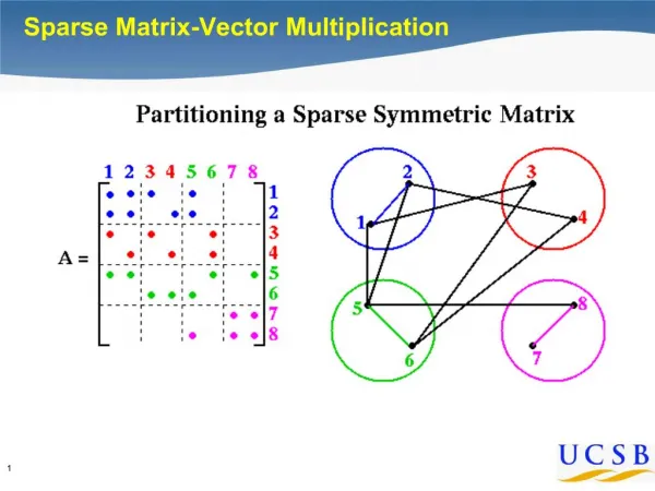
11. P0 P1 P2 P3 x P0 P1 P2 P3 y Conjugate gradient: Parallel implementation • Lay out matrix and vectors by rows • Hard part is matrix-vector producty = A*x • Algorithm Each processor j: Broadcast x(j) Compute y(j) = A(j,:)*x • May send more of x than needed • Partition / reorder matrix to reduce communication

12. (Matlab demo) • 2-way partition of eppstein mesh • 8-way dice of eppstein mesh

13. Preconditioners • Suppose you had a matrix B such that: • condition number κ(B-1A) is small • By = z is easy to solve • Then you could solve (B-1A)x = B-1b instead of Ax = b • B = A is great for (1), not for (2) • B = I is great for (2), not for (1) • Domain-specific approximations sometimes work • B = diagonal of A sometimes works • Or, bring back the direct methods technology. . .

14. (Matlab demo) • bcsstk08 with diagonal precond

15. x A RT R Incomplete Cholesky factorization (IC, ILU) • Compute factors of A by Gaussian elimination, but ignore fill • Preconditioner B = RTR  A, not formed explicitly • Compute B-1z by triangular solves (in time nnz(A)) • Total storage is O(nnz(A)), static data structure • Either symmetric (IC) or nonsymmetric (ILU)

16. (Matlab demo) • bcsstk08 with ic precond

17. 1 4 1 4 3 2 3 2 Incomplete Cholesky and ILU: Variants • Allow one or more “levels of fill” • unpredictable storage requirements • Allow fill whose magnitude exceeds a “drop tolerance” • may get better approximate factors than levels of fill • unpredictable storage requirements • choice of tolerance is ad hoc • Partial pivoting (for nonsymmetric A) • “Modified ILU” (MIC): Add dropped fill to diagonal of U or R • A and RTR have same row sums • good in some PDE contexts

18. Incomplete Cholesky and ILU: Issues • Choice of parameters • good: smooth transition from iterative to direct methods • bad: very ad hoc, problem-dependent • tradeoff: time per iteration (more fill => more time)vs # of iterations (more fill => fewer iters) • Effectiveness • condition number usually improves (only) by constant factor (except MIC for some problems from PDEs) • still, often good when tuned for a particular class of problems • Parallelism • Triangular solves are not very parallel • Reordering for parallel triangular solve by graph coloring

19. (Matlab demo) • 2-coloring of grid5(15)

20. A B-1 Sparse approximate inverses • Compute B-1 A explicitly • Minimize || B-1A – I ||F (in parallel, by columns) • Variants: factored form of B-1, more fill, . . • Good: very parallel • Bad: effectiveness varies widely

21. Support graph preconditioners: example [Vaidya] • A is symmetric positive definite with negative off-diagonal nzs • B is a maximum-weight spanning tree for A (with diagonal modified to preserve row sums) • factor B in O(n) space and O(n) time • applying the preconditioner costs O(n) time per iteration G(A) G(B)

22. Support graph preconditioners: example • support each edge of A by a path in B • dilation(A edge) = length of supporting path in B • congestion(B edge) = # of supported A edges • p = max congestion, q = max dilation • condition number κ(B-1A) bounded by p·q (at most O(n2)) G(A) G(B)

23. Support graph preconditioners: example • can improve congestion and dilation by adding a few strategically chosen edges to B • cost of factor+solve is O(n1.75), or O(n1.2) if A is planar • in recent experiments [Chen & Toledo], often better than drop-tolerance MIC for 2D problems, but not for 3D. G(A) G(B)

24. Domain decomposition (introduction) • Partition the problem (e.g. the mesh) into subdomains • Use solvers for the subdomains B-1 andC-1 to precondition an iterative solver on the interface • Interface system is the Schur complement: S = G – ET B-1E –FT C-1F • Parallelizes naturally by subdomains A =

25. (Matlab demo) • grid and matrix structure for overlapping 2-way partition of eppstein

26. Multigrid (introduction) • For a PDE on a fine mesh, precondition using a solution on a coarser mesh • Use idea recursively on hierarchy of meshes • Solves the model problem (Poisson’s eqn) in linear time! • Often useful when hierarchy of meshes can be built • Hard to parallelize coarse meshes well • This is just the intuition – lots of theory and technology

27. Other Krylov subspace methods • Nonsymmetric linear systems: • GMRES: for i = 1, 2, 3, . . . find xi  Ki (A, b) such that ri= (Axi – b)  Ki (A, b)But, no short recurrence => save old vectors => lots more space • BiCGStab, QMR, etc.:Two spaces Ki (A, b)and Ki (AT, b)w/ mutually orthogonal basesShort recurrences => O(n) space, but less robust • Convergence and preconditioning more delicate than CG • Active area of current research • Eigenvalues: Lanczos (symmetric), Arnoldi (nonsymmetric)

28. Direct A = LU Iterative y’ = Ay More General Non- symmetric Symmetric positive definite More Robust More Robust Less Storage The Landscape of Sparse Ax=b Solvers

29. n1/2 n1/3 Complexity of direct methods Time and space to solve any problem on any well-shaped finite element mesh

30. n1/2 n1/3 Complexity of linear solvers Time to solve model problem (Poisson’s equation) on regular mesh