Autotuning sparse matrix kernels
Autotuning sparse matrix kernels. Richard Vuduc Center for Applied Scientific Computing (CASC) Lawrence Livermore National Laboratory February 28, 2007. Predictions (2003). Need for “autotuning” will increase over time

Autotuning sparse matrix kernels
E N D
Presentation Transcript
Autotuning sparse matrix kernels Richard Vuduc Center for Applied Scientific Computing (CASC) Lawrence Livermore National Laboratory February 28, 2007
Predictions (2003) • Need for “autotuning” will increase over time • Improve performance for given app & machine using automated experiments • Example: Sparse matrix-vector multiply (SpMV), 1987 to present • Untuned: 10% of peak or less, decreasing • Tuned: 2x speedup, increasing over time • Tuning is getting harder (qualitative) • More complex machines & workloads • Parallelism
Is tuning getting easier? // y <-- y + A*x for all A(i,j): y(i) += A(i,j) * x(j) // Compressed sparse row (CSR) for each row i: t = 0 for k=ptr[i] to ptr[i+1]-1: t += A[k] * x[J[k]] y[i] = t • Exploit 8x8 dense blocks • As r x c, Mflop/s
Mflop/s (31.1%) Reference Mflop/s (7.6%) Speedups on Itanium 2: The need for search
Mflop/s (31.1%) Best: 4x2 Reference Mflop/s (7.6%) Speedups on Itanium 2: The need for search
Better, worse, or about the same?Itanium 2, 900 MHz 1.3 GHz
Better, worse, or about the same?Itanium 2, 900 MHz 1.3 GHz * Reference improves *
Better, worse, or about the same?Itanium 2, 900 MHz 1.3 GHz * Best possible worsens slightly *
Better, worse, or about the same?Pentium M Core 2 Duo (1-core)
Better, worse, or about the same?Pentium M Core 2 Duo (1-core) * Reference & best improve; relative speedup improves (~1.4 to 1.6) *
Better, worse, or about the same?Pentium M Core 2 Duo (1-core) * Note: Best fraction of peak decreased from 11% 9.6% *
Better, worse, or about the same?Power4 Power5 * Reference worsens! *
Better, worse, or about the same?Power4 Power5 * Relative importance of tuning increases *
A framework for performance tuningSource: SciDAC Performance Engineering Research Institute (PERI)
Outline • Motivation • OSKI: An autotuned sparse kernel library • Application-specific optimization “in the wild” • Toward end-to-end application autotuning • Summary and future work
Outline • Motivation • OSKI: An autotuned sparse kernel library • Application-specific optimization “in the wild” • Toward end-to-end application autotuning • Summary and future work
OSKI: Optimized Sparse Kernel Interface • Autotuned kernels for user’s matrix & machine • BLAS-style interface: mat-vec (SpMV), tri. solve (TrSV), … • Hides complexity of run-time tuning • Includes fast locality-aware kernels: ATA*x, … • Faster than standard implementations • Standard SpMV < 10% peak, vs. up to 31% with OSKI • Up to 4x faster SpMV, 1.8x TrSV, 4xATA*x, … • For “advanced” users & solver library writers • PETSc extension available (OSKI-PETSc) • Kokkos (for Trilinos) by Heroux • Adopted by ClearShape, Inc. for shipping product (2x speedup)
Tunable matrix-specific optimization techniques • Optimizations for SpMV • Register blocking (RB): up to 4x over CSR • Variable block splitting: 2.1x over CSR, 1.8x over RB • Diagonals: 2x over CSR • Reordering to create dense structure + splitting: 2x over CSR • Symmetry: 2.8x over CSR, 2.6x over RB • Cache blocking: 3x over CSR • Multiple vectors (SpMM): 7x over CSR • And combinations… • Sparse triangular solve • Hybrid sparse/dense data structure: 1.8x over CSR • Higher-level kernels • AAT*x, ATA*x: 4x over CSR, 1.8x over RB • A*x: 2x over CSR, 1.5x over RB
Tuning for workloads • Bi-conjugate gradients - equal mix of A*x and AT*y • 3x1: Ax, ATy = 1053, 343 Mflop/s 517 Mflop/s • 3x3: Ax, ATy = 806, 826 Mflop/s 816 Mflop/s • Higher-level operation - (Ax, ATy) kernel • 3x1: 757 Mflop/s • 3x3: 1400 Mflop/s • Matrix powers (Ak*x) with data structure transformations • A2*x: up to 2x faster • New latency-tolerant solvers? (Hoemmen’s thesis, on-going at UCB)
How OSKI tunes (Overview) Application Run-Time Library Install-Time (offline)
How OSKI tunes (Overview) Application Run-Time Library Install-Time (offline) 1. Build for Target Arch. 2. Benchmark Generated code variants Benchmark data
How OSKI tunes (Overview) Application Run-Time Library Install-Time (offline) 1. Build for Target Arch. 2. Benchmark Workload from program monitoring History Matrix Generated code variants Benchmark data 1. Evaluate Models Heuristic models
How OSKI tunes (Overview) Extensibility: Advanced users may write & dynamically add “Code variants” and “Heuristic models” to system. Application Run-Time Library Install-Time (offline) 1. Build for Target Arch. 2. Benchmark Workload from program monitoring History Matrix Generated code variants Benchmark data 1. Evaluate Models Heuristic models 2. Select Data Struct. & Code To user: Matrix handle for kernel calls
Examples of OSKI’s early impact • Early adopter: ClearShape, Inc. • Core product: lithography simulator • 2x speedup on full simulation after using OSKI • Proof-of-concept: SLAC T3P accelerator cavity design simulator • SpMV dominates execution time • Symmetry, 2x2 block structure • 2x speedups
Strengths and limitations of the library approach • Strengths • Isolates optimization in the library for portable performance • Exploits domain-specific information aggressively • Handles run-time tuning naturally • Limitations • “Generation Me”: What about my application and its abstractions? • Run-time tuning: run-time overheads • Limited context for optimization (without delayed evaluation) • Limited extensibility (fixed interfaces)
Outline • Motivation • OSKI: An autotuned sparse kernel library • Application-specific optimization “in the wild” • Toward end-to-end application autotuning • Summary and future work
Tour of application-specific optimizations • Five case studies • Common characteristics • Complex code • Heavy use of abstraction • Use generated code (e.g., SWIG C++/Python bindings) • Benefit from extensive code and data restructuring • Multiple bottlenecks
[1] Loop transformations for SMG2000 • SMG2000, implements semi-coarsening multigrid on structured grids (ASC Purple benchmark) • Residual computation has an SpMV bottleneck • Loop below looks simple but non-trivial to extract for (si = 0; si < NS; ++si) for (k = 0; k < NZ; ++k) for (j = 0; j < NY; ++j) for (i = 0; i < NX; ++i) r[i + j*JR + k*KR] -= A[i + j*JA + k*KA + SA[si]] * x[i + j*JX + k*KX + Sx[si]]
[1] Before transformation for (si = 0; si < NS; si++) /* Loop1 */ for (kk = 0; kk < NZ; kk++) { /* Loop2 */ for (jj = 0; jj < NY; jj++) { /* Loop3 */ for (ii = 0; ii < NX; ii++) { /* Loop4 */ r[ii + jj*Jr + kk*Kr] -= A[ii + jj*JA + kk*KA + SA[si]] * x[ii + jj*JA + kk*KA + SA[si]]; } /* Loop4 */ } /* Loop3 */ } /* Loop2 */ } /* Loop1 */
[1] After transformation, including interchange, unrolling, and prefetching for (kk = 0; kk < NZ; kk++) { /* Loop2 */ for (jj = 0; jj < NY; jj++) { /* Loop3 */ for (si = 0; si < NS; si++) { /* Loop1 */ double* rp = r + kk*Kr + jj*Jr; const double* Ap = A + kk*KA + jj*JA + SA[si]; const double* xp = x + kk*Kx + jj*Jx + Sx[si]; for (ii = 0; ii <= NX-3; ii += 3) { /* core Loop4 */ _mm_prefetch (Ap + PFD_A, _MM_HINT_NTA); _mm_prefetch (xp + PFD_X, _MM_HINT_NTA); rp[0] -= Ap[0] * xp[0]; rp[1] -= Ap[1] * xp[1]; rp[2] -= Ap[2] * xp[2]; rp += 3; Ap += 3; xp += 3; } /* core Loop4 */ for ( ; ii < NX; ii++) { /* fringe Loop4 */ rp[0] -= Ap[0] * xp[0]; rp++; Ap++; xp++; } /* fringe Loop4 */ } /* Loop1 */ } /* Loop3 */ } /* Loop2 */
[1] Loop transformations for SMG2000 • 2x speedup on kernel from specialization, loop interchange, unrolling, prefetching • But only 1.25x overall---multiple bottlenecks • Lesson: Need complex sequences of transformations • Use profiling to guide • Inspect run-time data for specialization • Transformations are automatable • Research topic: Automated specialization of hypre?
Accelerator design code from SLAC calcBasis() very expensive Scaling problems as |Eigensystem| grows In principle, loop interchange or precomputation via slicing possible /* Post-processing phase */ foreach mode in Eigensystem foreach elem in Mesh b = calcBasis (elem) f = calcField (b, mode) [2] Slicing and dicing W3P
Accelerator design code calcBasis() very expensive Scaling problems as |Eigensystem| grows In principle, loop interchange or precomputation via slicing possible Challenges in practice “Loop nest” ~ 500+ LOC 150+ LOC to calcBasis() calcBasis() in 6-deep call chain, 4-deep loop nest, 2 conditionals File I/O Changes must be unobtrusive /* Post-processing phase */ foreach mode in Eigensystem foreach elem in Mesh // { … b = calcBasis (elem) // } f = calcField (b, mode) writeDataToFiles (…); [2] Slicing and dicing W3P
[2] W3P: Impact and lessons • 4-5x speedup for post-processing step; 1.5x overall • Changes “checked-in” • Lesson: Need clean source-level transformations • To automate, need robust program analysis and developer guidance • Research: Annotation framework for developers • [w/ Quinlan, Schordan, Yi: POHLL’06]
[3] Structure splitting • Convert (array of structs) into (struct of arrays) • Improve spatial locality through increased stride-1 accesses • Make code hardware-prefetch and vector/SIMD unit “friendly”c struct Type { double p; double x, y, z; double E; int k; } X[N], Y[N]; for (i = 0; i < N; i++) Y[i].E += Y[X[i].k].p; double Xp[N]; double Xx[N], Xy[N], Xz[N]; double XE[N]; int Xk[N]; // … same for Y … for (i = 0; i < N; i++) YE[i] += sqrt (Yp[Xk[i]]);
[3] Structure splitting: Impact and challenges • 2x speedup on a KULL benchmark (suggested by Brian Miller) • Implementation challenges • Potentially affects entire code • Can apply only locally, at a cost • Extra storage • Overhead of copying • Tedious to do by hand • Lesson: Extensive data restructuring may be necessary • Research: When and how best to split?
[4] Finding a loop-fusion needle in a haystack • Interprocedural loop fusion finder [w/ B. White : Cornell U.] • Known example had 2x speedup on benchmark (Miller) • Built “abstraction-aware” analyzer using ROSE • First pass: Associate “loop signatures” with each function • Second pass: Propagate signatures through call chains for (Zone::iterator z = zones.begin (); z != zones.end (); ++z) for (Corner::iterator c = (*z).corners().begin (); …) for (int s = 0; s < c->sides().size(); s++) …
[4] Finding a loop-fusion needle in a haystack • Found 6 examples of 3- and 4-deep nested loops • “Analysis-only” tool • Finds, though does not verify/transform • Lesson: “Classical” optimizations relevant to abstraction use • Research • Recognizing and optimizing abstractions [White’s thesis, on-going] • Extending traditional optimizations to abstraction use
[5] Aggregating messages (on-going) • Idea: Merge sends (suggested by Miller) DataType A; // … operations on A … A.allToAll(); // … DataType B; // … operations on B … B.allToAll(); DataType A; // … operations on A … // … DataType B; // … operations on B … bulkAllToAll(A, B); • Implementing a fully automated translator to find and transform • Research: When and how best to aggregate?
Summary of application-specific optimizations • Like library-based approach, exploit knowledge for big gains • Guidance from developer • Use run-time information • Would benefit from automated transformation tools • Real code is hard to process • Changes may become part of software re-engineering • Need robust analysis and transformation infrastructure • Range of tools possible: analysis and/or transformation • No silver bullets or magic compilers
Outline • Motivation • OSKI: An autotuned sparse kernel library • “Real world” optimization • Toward end-to-end application autotuning • Summary and future work

