Sparse Matrix Algorithms
Sparse Matrix Algorithms. CS 524 – High-Performance Computing. Sparse Matrices. Sparse matrices have the majority of their elements equal to zero

Sparse Matrix Algorithms
E N D
Presentation Transcript
Sparse Matrix Algorithms CS 524 – High-Performance Computing
Sparse Matrices • Sparse matrices have the majority of their elements equal to zero • More significantly, a matrix is considered sparse if a computation involving it can utilize the number and location of its nonzero elements to reduce the run time over the same computation on a dense matrix of the same size. • The finite difference and finite element methods for solving partial differential equations arising from mathematical models of continuous domain require sparse matrix algorithms. • For many problems, it is not necessary to explicitly assemble the sparse matrices. Rather, operations are done using specialized data structures. CS 524 (Wi 2003/04)- Asim Karim @ LUMS
Storage Schemes for Sparse Matrices • Store only the nonzero elements and their locations in the matrix • Saves memory, as storage used can be much less than n2 • May improve performance • Several storage schemes and data structures are available. Some may be better than others for a given algorithm. • Common storage schemes • Coordinate format • Compressed sparse row format (CSR format) • Diagonal storage format • Ellpack-Itpack format • Jagged-diagonal format CS 524 (Wi 2003/04)- Asim Karim @ LUMS
Coordinate Format • VAL is q x 1 array of nonzero elements (in any order) • I is q x 1 array of ith coordinate of element • J is q x 1 array of jth coordinate of element CS 524 (Wi 2003/04)- Asim Karim @ LUMS
Compressed Sparse Row (CSR) Format • VAL is q x 1 array of nonzero elements stored in the order of their rows (however, within a row they can be stored in any order) • J is q x 1 array of the column number of each nonzero element • I is n x 1 array that points to the first entry of the ith row in VAL and J CS 524 (Wi 2003/04)- Asim Karim @ LUMS
Diagonal Storage Format • VAL is n x d array of nonzero elements in diagonals; d = # of diagonals (order of diagonals in VAL is not important) • OFFSET is d x 1 array of offset of diagonal from principal diagonal • Banded format: Uses VAL and parameters for thickness of band and its lower (or upper) limit. CS 524 (Wi 2003/04)- Asim Karim @ LUMS
Ellpack-Itpack Format • VAL is n x m array of nonzero elements in rows; m = max. # of nonzero elements in a row • J is n x m array of column number of corresponding entry in VAL. A indicator value is used to indicate the end of a row CS 524 (Wi 2003/04)- Asim Karim @ LUMS
Jagged-Diagonal Format (1) CS 524 (Wi 2003/04)- Asim Karim @ LUMS
Jagged-Diagonal Format (2) • Rows in matrix are ordered in decreasing number of nonzero elements • VAL is q x 1 array of nonzero elements in each row in increasing column order. That is, the first nonzero element in each row is stored contiguously, then the second, and so on. • J is q x 1 array of column number of corresponding entries in VAL • I is m x 1 array of pointers to beginning of each jagged diagonal CS 524 (Wi 2003/04)- Asim Karim @ LUMS
Vector Inner Product – p <= n • y = xTx; x is a n x 1 vector and y is a scalar • Data partitioning: Each processor has n/p elements of x • Communication: global reduction sum of y (scalar) • Computation: n/p multiplications + additions • Parallel run time: Tp = 2tcn/p + (ts + tw) • Algorithm is cost-optimal, as sequential and parallel cost is O(n) when p = O(n) CS 524 (Wi 2003/04)- Asim Karim @ LUMS
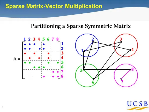
Sparse Matrix-Vector Multiplication • y = Ax, where A is sparse n x n matrix; x and y are vectors of dimension n • Sparse MVM algorithms depend on the structure of the sparse matrix and the storage scheme used • In many MVMs arising in science and engineering (e.g. from FDM solution of PDEs) the matrix has a block-tridiagonal structure • Other common sparse matrix structures include banded sparse matrices and general unstructured matrices CS 524 (Wi 2003/04)- Asim Karim @ LUMS
Block-Tridiagonal Matrix CS 524 (Wi 2003/04)- Asim Karim @ LUMS
Striped Partitioning – p <= n (1) • Data partitioning: Each processor has n/p rows of A and n/p elements of x • Three components of the multiplication • Multiplication of principal diagonal. This requires no communication. • Multiplication of adjacent off-diagonals. These require exchange of border elements of vector x • Multiplication of outer block diagonals. These require communication of vector x depending on n and p CS 524 (Wi 2003/04)- Asim Karim @ LUMS
Striped Partitioning – p <= n (2) CS 524 (Wi 2003/04)- Asim Karim @ LUMS
Striped Partitioning – p <= n (3) • Communication • Exchange of border elements of vector x • When p ≤ √n, exchange of √n elements of vector x between neighboring processors • When p > √n, Pi exchanges n/p elements of vector x with processors with index i ± p/√n • Computation: Except for the first and last √n rows, there are 5 nonzero elements. Thus, at most 5 multiplications + additions are needed per row CS 524 (Wi 2003/04)- Asim Karim @ LUMS
Striped Partitioning – p <= n (4) • Parallel run time when p ≤ √n • Tp = 10tcn/p + 2[ts + tw√n] • Parallel run time when p > √n • Tp = 10tcn/p + 2[ts + tw] + 2[ts + twn/p] CS 524 (Wi 2003/04)- Asim Karim @ LUMS
Partitioning the Grid (1) CS 524 (Wi 2003/04)- Asim Karim @ LUMS
Partitioning the Grid (2) • Data partitioning: Each processor has √(n/p) x √(n/p) rows of matrix A and √(n/p) x √(n/p) elements of vector x corresponding to the grid points • Communication: Exchange of vector elements corresponding to the √(n/p) grid points with neighbors • Parallel run time: Tp = 10tcn/p + 4[ts + tw√(n/p)] CS 524 (Wi 2003/04)- Asim Karim @ LUMS
Iterative Methods for Sparse Linear Systems • Popular methods for solving sparse linear systems, Ax = b • Generates a sequence of approximations to vector x that converges to the solution of the system • Characteristics • Number of iterations required is problem data dependent • Each iteration requires a matrix-vector multiplication • Generally faster than direct methods • Appropriate for sparse coefficient matrices • Methods • Jacobi iterative • Gauss-Seidel and SOR • Conjugate gradient and preconditioned CG CS 524 (Wi 2003/04)- Asim Karim @ LUMS
Jacobi Iterative Method • Simple iterative procedure that is guaranteed to converge for diagonally dominated systems xk(i) = A-1(i,i)[b(i) – ΣA(i,j)xk-1(j)] Or xk(i) = rk-1(i)/A(i,i) + xk-1(i) • rk-1 is the residual at the k-1 iteration • rk-1 = b(i) – ΣA(i,j)xk-1(j) CS 524 (Wi 2003/04)- Asim Karim @ LUMS
Finite Difference Discretization Linearized order of unknowns in a 2-D grid Only internal grid points are unknown j = N+1 13 14 15 16 j = 4 j = 3 j = 2 1 2 3 4 j = 1 j = 1 j = 0 i = 0 i = 2 i = N+1 i = 1 i = 4 i = 1 i = 3 CS 524 (Wi 2003/04)- Asim Karim @ LUMS
Jacobi Iterative Method – Sequential for (iter = 0; iter < maxiter; iter++) { for (i = 1; i <= N; i++) { for (j = 1; j <= N; j++) { xnew[i][j] = b[i][j] - odiag*(xold[i-1][j] + xold[i+1][j] + xold[i][j-1] + xold[i][j+1]); xnew[i][j] = xnew[i][j]/diag; } } for (i = 1; i <= N; i++) { for (j = 1; j <= N; j++) resid[i][j] = b[i][j] - diag*xnew[i][j] \ - odiag*(xnew[i-1][j]+xnew[i+1][j]+xnew[i][j-1]+xnew[i][j+1]); } for (i = 1; i <= N; i++) { for (j = 1; j <= N; j++) xold[i][j] = xnew[i][j]; } } CS 524 (Wi 2003/04)- Asim Karim @ LUMS
Conjugate Gradient Method • Powerful iterative method for systems in which A is symmetric positive definite, i.e, xTAx > 0 for any nonzero vector x • Formulates the problem as a minimization problem • Solution of the system is found by minimizing q(x) = (1/2)xTAx – xTb • Iteration • xk = xk-1 + αkpk • rk = rk-1 – αkApk • p1 = r0 = b; pk+1 = rk + ||rk||2pk/||rk-1||2 • αk = ||rk-1||2/(pk)TApk CS 524 (Wi 2003/04)- Asim Karim @ LUMS
CG Method – Sequential (1) for (iter = 1; iter <= maxiter; iter++) { // Form v = Ap for (i = 1; i <= N; i++) { for (j = 1; j <= N; j++) v[i][j] = odiag*(p[i-1][j] + p[i+1][j] + p[i][j-1] + p[i][j+1]) + diag*p [i][j]; } // Form (r dot r), (v dot p) and a rdotr = 0.0; pdotv = 0.0; for (i = 1; i <= N; i++) { for (j = 1; j <= N; j++) { rdotr = rdotr + r[i][j]*r[i][j]; pdotv = pdotv + p[i][j]*v[i][j]; } } a = rdotr/pdotv; CS 524 (Wi 2003/04)- Asim Karim @ LUMS
CG Method – Sequential (2) // Update x and compute new residual rnew for (i = 1; i <= N; i++) { for (j = 1; j <= N; j++) { x[i][j] = x[i][j] + a*p[i][j]; rnew[i][j] = r[i][j] - a*v[i][j]; }} // Compute new residual and g rndotrn = 0.0; for (i = 1; i <= N; i++) { for (j = 1; j <= N; j++) rndotrn = rndotrn + rnew[i][j]*rnew[i][j]; } rhonew = sqrt(rndotrn); g = rndotrn/rdotr; // Compute new search direction p, and move rnew into r for (i = 1; i <= N; i++) { for (j = 1; j <= N; j++) { p[i][j] = rnew[i][j] + g*p[i][j]; r[i][j] = rnew[i][j]; }} CS 524 (Wi 2003/04)- Asim Karim @ LUMS