Sparse Matrix Computations
Sparse Matrix Computations. CSCI 317 Mike Heroux. Matrices. Matrix (defn): (not rigorous) An m -by- n , 2 dimensional array of numbers. Examples: . 1.0 2.0 1.5 A = 2.0 3.0 2.5 1.5 2.5 5.0. a 11 a 12 a 13 A = a 21 a 22 a 23 a 31 a 32 a 33. Sparse Matrices.

Sparse Matrix Computations
E N D
Presentation Transcript
Sparse Matrix Computations CSCI 317 Mike Heroux CSCI 317 Mike Heroux
Matrices • Matrix (defn): (not rigorous) An m-by-n, 2 dimensional array of numbers. • Examples: 1.0 2.0 1.5 A = 2.0 3.0 2.5 1.5 2.5 5.0 a11a12a13 A = a21a22a23 a31a32a33 CSCI 317 Mike Heroux
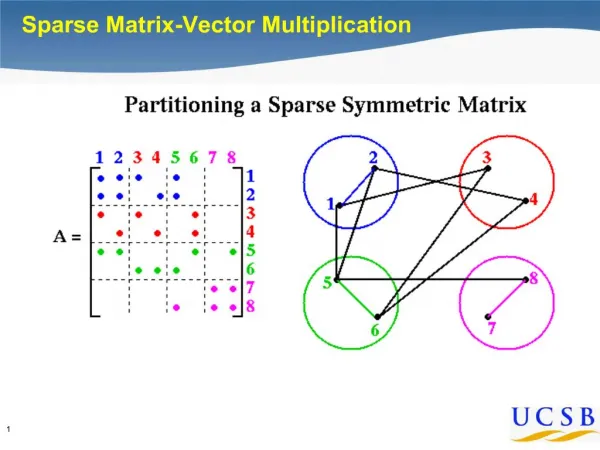
Sparse Matrices • Sparse Matrix (defn): (not rigorous) An m-by-n matrix with enough zero entries that it makes sense to keep track of what is zero and nonzero. • Example: a11a120 0 0 0 a21a22a23 0 0 0 A = 0 a32a33 a34 0 0 0 0 a43 a44a45 0 0 0 0 a54a55a56 0 0 0 0 a65a66 CSCI 317 Mike Heroux
Dense vs Sparse Costs • What is the cost of storing the tridiagonal matrix with all entries? • What is the cost if we store each of the diagonals as vector? • What is the cost of computing y = Ax for vectors x (known) and y (to be computed): • If we ignore sparsity? • If we take sparsity into account? CSCI 317 Mike Heroux
Origins of Sparse Matrices • In practice, most large matrices are sparse. Specific sources: • Differential equations. • Encompasses the vast majority of scientific and engineering simulation. • E.g., structural mechanics. • F = ma. Car crash simulation. • Stochastic processes. • Matrices describe probability distribution functions. • Networks. • Electrical and telecommunications networks. • Matrix element aij is nonzero if there is a wire connecting point i to point j. • And more… CSCI 317 Mike Heroux
Example: 1D Heat Equation (Laplace Equation) • The one-dimensional, steady-state heat equation on the interval [0,1] is as follows: • The solution u(x), to this equation describes the distribution of heat on a wire with temperature equal to a and b at the left and right endpoints, respectively, of the wire. CSCI 317 Mike Heroux
Finite Difference Approximation • The following formula provides an approximation of u”(x) in terms of u: • For example if we want to approximate u”(0.5) with h = 0.25: CSCI 317 Mike Heroux
1D Grid • Note that it is impossible to find u(x) for all values of x. • Instead we: • Create a “grid” with n points. • Then find an approximate to u at these grid points. • If we want a better approximation, we increase n. u(0)=a = u0 u(1)=b = u4 u(0.25)=u1 u(0.5)=u2 u(0.75)=u3 u(x): Interval: x: x0= 0 x1= 0.25 x2= 0.5 x3= 0.75 x4= 1 Note: • We know u0 and u4 . • We know a relationship between the ui via the finite difference equations. • We need to find uifor i=1, 2, 3. CSCI 317 Mike Heroux
What We Know CSCI 317 Mike Heroux
Write in Matrix Form This is a linear system with 3 equations and three unknowns. We can easily solve. Note that n=5 generates this 3 equation system. In general, for n grid points on [0, 1], we will have n-2 equations and unknowns. CSCI 317 Mike Heroux
General Form of 1D Finite Difference Matrix CSCI 317 Mike Heroux
A View of More Realistic Problems • The previous example is very simple. • But basic principles apply to more complex problems. • Finite difference approximations exist for any differential equation. • Leads to far more complex matrix patterns. • For example… CSCI 317 Mike Heroux
“Tapir” Matrix (John Gilbert) CSCI 317 Mike Heroux
Corresponding Mesh CSCI 317 Mike Heroux
Sparse Linear Systems:Problem Definition • A frequent requirement for scientific and engineering computing is to solve: Ax = b where A is a known large (sparse) matrix a linear operator, b is a known vector, x is an unknown vector. NOTE:We are using x differently than before. Previous x: Points in the interval [0, 1]. New x: Vector of u values. • Goal: Find x. • Method: We will look at two different methods: Jacobi and Gauss-Seidel. CSCI 317 Mike Heroux
Iterative Methods • Given an initial guess for x, called x(0), (x(0) = 0 is acceptable) compute a sequence x(k), k = 1,2, … such that each x(k) is “closer” to x. • Definition of “close”: • Suppose x(k) = x exactly for some value of k. • Then r(k) = b – Ax(k) = 0 (the vector of all zeros). • And norm(r(k)) = sqrt(<r(k), r(k)>) = 0 (a number). • For any x(k), let r(k) = b – Ax(k) • If norm(r(k)) = sqrt(<r(k), r(k)>) is small (< 1.0E-6 say) then we say that x(k) is close to x. • The vector r is called the residual vector. CSCI 317 Mike Heroux
linear operator applications vector-vector operations Scalar operations scalar product <x,y> defined by vector space Linear Conjugate Gradient Methods Types of operations Types of objects Linear Conjugate Gradient Algorithm CSCI 317 Mike Heroux
General Sparse Matrix • Example: a110 0 0 0 a16 0 a22a23 0 0 0 A = 0 a32a33 0 a35 0 0 0 0 a440 0 0 0 a53 0 a55a56 a61 0 0 0 a65a66 CSCI 317 Mike Heroux
Compressed Row Storage (CRS) Format Idea: • Create 3 length m arrays of pointers 1 length m array of ints : double ** values = new double *[m]; double ** diagonals = new double*[m]; int ** indices = new int*[m]; int * numEntries = new int[m]; CSCI 317 Mike Heroux
Compressed Row Storage (CRS) Format Fill arrays as follows: for (i=0; i<m; i++) { // for each row numEntries[i] = numRowEntries, number of nonzero entries in row i. values[i] = new double[numRowEntries]; indices[i] = new int[numRowEntries]; for (j=0; j<numRowEntries; j++) { // for each entry in row i values[i][j] = value of jth row entry. indices[i][j] = column index of jth row entry. if (i==column index) diagonal[i] = &(values[i][j]); } } CSCI 317 Mike Heroux
CRS Example (diagonal omitted) CSCI 317 Mike Heroux
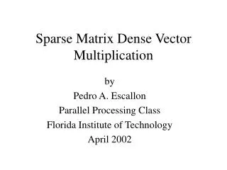
Matrix, Scalar-Matrix andMatrix-Vector Operations • Given vectors w, x and y, scalars alpha and beta and matrices A and B we define: • matrix trace: • alpha = tr(A)α= a11 + a22 + ...+ ann • matrix scaling: • B = alpha * Abij = α aij • matrix-vector multiplication (with update): • w = alpha * A * x + beta * y wi = α(ai1 x1 + ai2 x2 + ...+ ainxn) + βyi CSCI 317 Mike Heroux
Common operations (See your notes) • Consider the following operations: • Matrix trace. • Matrix scaling. • Matrix-vector product. • Write mathematically and in C/C++. CSCI 317 Mike Heroux
Complexity • (arithmetic) complexity (defn) The total number of arithmetic operations performed using a given algorithm. • Often a function of one or more parameters. • parallel complexity(defn) The number parallel operations performed assuming an infinite number of processors. CSCI 317 Mike Heroux
Complexity Examples (See your notes) • What is the complexity of: • Sparse Matrix trace? • Sparse Matrix scaling. • Sparse Matrix-vector product? • What is the parallel complexity of these operations? CSCI 317 Mike Heroux