Introduction to DNA Microarrays
390 likes | 678 Views
Introduction to DNA Microarrays. DNA Microarrays and DNA chips resources on the web. INTRODUCTION. Microarray analysis is a new technology which allows scientists to detect thousands of genes in a small sample simultaneously and to analyze the expression of those genes.

Introduction to DNA Microarrays
E N D
Presentation Transcript
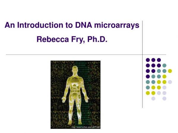
Introduction to DNA Microarrays DNA Microarrays and DNA chips resources on the web
INTRODUCTION Microarray analysis is a new technology which allows scientists to detect thousands of genes in a small sample simultaneously and to analyze the expression of those genes. Microarrays are simply ordered sets of DNA molecules of known sequence. Usually rectangular, they can consist of a few hundred to hundreds of thousands of sets. Each individual feature goes on the array at precisely defined location on the substrate.
Potential application domains • Identification of complex genetic diseases • Drug discovery and toxicology studies • Mutation/polymorphism detection (SNP’s) • Pathogen analysis • Differing expression of genes over time, between tissues, and disease states • Preventive medicine • Ability to subtype disease and design drugs that treat disease causes, rather than symptoms • Specific genotype (population) targeted drugs • More targeted drug treatments – AIDS • Genetic testing and privacy
The technique Based on already known methods, such as fluorescence and hybridization. It's goal is to compare gene transcription in two or more different kinds of cells. There is four main steps in making an array experiment : 1- Array fabrication 2- Sample preparation and hybridization 3- Scanning the array 4- Exploring the results
The challenge The big revolution here is in the "micro" term. New slides will contain a survey of the human genome on a 2 cm2 chip! The use of this large-scale method tends to create phenomenal amounts of data, which have then to be stored, processed and analyzed. As the technique is quite new, analyzing the data is still a problem, and nothing is standardized yet. A few databases and on-line repositories are coming out, and the future standard will probably be chosen between these ones. This is a job for…Bioinformatics !
Course overview Theory : Introduction to the technique of microarrays Analyzing the data : a few methods Quick survey of tools, databases, datasets available on the web Practical : Using on-line tools for microarrays Searching public databases
THE EXPERIMENT : making the chip 1- Designing the chip : choosing genes of interest for the experiment - Selection of chip probes that represent the investigated genes. - Finding sequences, usually in the EST database. - Problems : sequencing errors, alternative splicing, chimeric sequences, contamination…
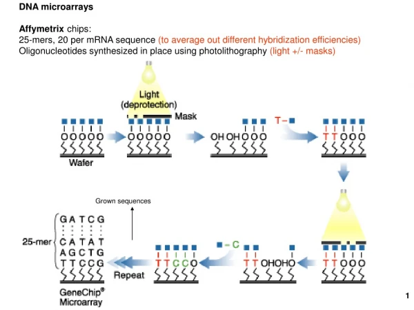
THE EXPERIMENT : making the chip • 2- Spotting the probes on the substrate • Substrate : usually glass, but also nylon membranes, plastic, ceramic… • Probes : cDNA probes (500-5000 nucleotides, dna chips), oligonucleotides (20~80-mer oligos, oligo chips), genomic DNA ( ~50’000 bases) • Printing methods : microspotting, ink-jetting (for dna chips) or in-situ printing, for example photolithography (for oligos, Affymetrix method)
THE EXPERIMENT : making the chip Microspotting and ink-jetting
THE EXPERIMENT : making the chip The microspotting and ink-jetting are done by a robot called “arrayer”
THE EXPERIMENT : making the chip Oligo-spotting (Affymetrix method)
THE EXPERIMENT : hybridization • Sample preparation • Extracting DNA (for genomic studies) or mRNA (for gene expressions studies) from the two samples to compare. • Target labeling. Making cDNAs with both extracts, and labeling them with different fluors to allow direct comparison.
THE EXPERIMENT : hybridization Samples are eluted on the chip, put in a hybridization chamber, and then washed.
THE EXPERIMENT : generating data • Chip scanning • Fluorescence measurements are made with scanning laser fluorescence microscope that illuminates each DNA spot and measures fluorescence for each dye separately. It creates one red and one green image. • The two images are then superimposed to give a virtual result of RNA amounts in both samples
THE EXPERIMENT : generating data Chip scanning
1- Samples 2- Extracting mRNA 3- Labeling 4- Hybridizing 5- Scanning 6- Visualizing
Examples of scanner outputs Affymetrix chip Stanford chip
THE EXPERIMENT : generating data • Image analysis • These fluorescence measures are then used to determine the ratio, and in turn the relative abundance, of the sequence of each specific gene in the two mRNA or DNA samples. • This analysis is performed by a software such as “scanalyze”, available at : http://rana.lbl.gov/EisenSoftware.htm • or “Spotfinder” from TIGR • The files created can then be submitted to further analysis
THE EXPERIMENT : making sense of the data Although the visual image of a microarray panel is alluring, its information content, per se, is still not readable. How can one visualize, organize and explore the meaning of information consisting of several million measurements of expression of thousands of genes under thousands of conditions?
THE EXPERIMENT : making sense of the data Data mining depends on the questions which are asked. The most frequent question is to find sets of genes that have correlated expression profiles (belonging to the same biological process and/or co-regulated), or to devide conditions to groups with similar gene expression profiles ( for example divide drugs according to their effect on gene expression. The method used to answer these questions is called CLUSTERING.
Clustering data • Input: N data points, Xi, i=1,2,…,N (the color ratios measured with Scanalyze, for example) in a D dimensional space. N and D will be either genes and conditions for gene clustering, or conditions and genes for conditions clustering. • Goal: Find “natural”groups or clusters. • Note: according to the method, the number of clusters will be fixed from the beginning (K-means) or determined after the analysis (hierarchical clustering)
Clustering data Before clustering, a few steps to “clean the data are necessary ( normalization, filtering) • Clustering methods : • 1- Agglomerative Hierarchical • 2- Centroids: K-means or SOM • 3- Super-Paramagnetic Clustering For a good introduction on different clustering techniques, read the article from Gavin Sherlock “Analysis of large-scale gene expression data” in Current Opinion in Immunology 2000, 12:201-205 (html,pdf)
2 4 5 3 1 1 3 2 4 5 Agglomerative Hierarchical Clustering Distance between joined clusters Dendrogram The dendrogram induces a linear ordering of the data points
Agglomerative Hierarchical Clustering Before doing a hierarchical clustering, one has to define two things : 1-The similarity measure between two genes (or experiments) Centered correlation Uncentered correlation Absolute correlation Euclidean 2- The distance measure between the new cluster and the others Single Linkage: distance between closest pair. Complete Linkage: distance between farthest pair. Average Linkage: distance between cluster centers
Centroid methods - K-means • Start with random position of K centroids. • Iteratre until centroids are stable • Assign points to centroids • Move centroids to centerof assign points Iteration = 0
Centroid Methods - K-means • Start with random position of K centroids. • Iteratre until centroids are stable • Assign points to centroids • Move centroids to centerof assign points Iteration = 1
Centroid Methods - K-means • Start with random position of K centroids. • Iteratre until centroids are stable • Assign points to centroids • Move centroids to centerof assign points Iteration = 3
Self-organizing Maps • Choose a number of partitions • Assign a random reference vector to each partition. • Pick a gene randomly and assign it to its most similar reference vector. • Adjust that reference vector is so that it is more similar to the chosen gene. • Adjust the other reference vectors. • Repeat thousands of times until partitions are stable. A self-organizing map.
Super-Paramagnetic Clustering (SPC)M.Blatt, S.Weisman and E.Domany (1996) Neural Computation • The idea behind SPC is based on the physical properties dilute magnets. • Calculating correlation between magnet orientations at different temperatures (T). T=Low
Super-Paramagnetic Clustering (SPC)M.Blatt, S.Weisman and E.Domany (1996) Neural Computation • The idea behind SPC is based on the physical properties dilute magnets. • Calculating correlation between magnet orientations at different temperatures (T). T=High
Super-Paramagnetic Clustering (SPC)M.Blatt, S.Weisman and E.Domany (1996) Neural Computation • The algorithm simulates the magnets behavior at a range of temperatures and calculates their correlation • The temperature (T) controls the resolution T=Intermediate
Clustering data Available clustering tools • M. Eisen’s programs for clustering and display of results (Cluster, TreeView) • Predefined set of normalizations and filtering • Agglomerative, K-means, 1D SOM • Matlab • Agglomerative, public m-files. • Dedicated software packages (SPC) • Web sites: e.g. http://ep.ebi.ac.uk/EP/EPCLUST/ • Statistical programs (SPSS, SAS, S-plus) • And much others …
Clustering data The final data representation is then a big matrix with rows being the genes and columns representing the different experiments. To keep the image coherent with the scan output, the ratio numbers calculated by Scanalyze are transformed back in color spots on a green-red based scale.
Clustering data Another way to represent these data is a graph showing the gene’s expression variation during the different experiments Expression variation of nine genes along the 19 experiments from Lyer et al. (Fibroblast response to serum stimulation)