DNA Microarrays
DNA Microarrays. Eran Segal Weizmann Institute. Microarray History. 1991: Photolithographic printing (Affymetrix) 1994: First cDNA collections developed at Stanford 1995: Quantitative monitoring of gene expression patterns with a complementary DNA microarray

DNA Microarrays
E N D
Presentation Transcript
DNA Microarrays Eran Segal Weizmann Institute
Microarray History • 1991: Photolithographic printing (Affymetrix) • 1994: First cDNA collections developed at Stanford • 1995: Quantitative monitoring of gene expression patterns with a complementary DNA microarray • 1996: Commercialization of arrays (Affymetrix) • 1997: Genome-wide expression monitoring in yeast • 2000: Portraits/ Signatures of cancer • 2003: Introduction into clinical practices • 2004: Whole human genome on one microarray
Tiling Microarrays • Affymetrix: 6 million 25-mer probes, non-custom • Agilent: 244K 60-mer probes, customizable • Nimblegen: 1.2M 60-mer probes, customizable • Applications • ChIP-chip • DNA methylation • Nucleosome localization • Copy number variation and CGH • Transcriptome mapping
Microarray Biases • Probe intensity depends on probe sequence • GC content is a major predictor of signal intensity • Nucleotide position on the probe • Nucleotides further away from the glass can bind with greater efficiency • Self-complementarity of probe • Probes may form secondary structures and be less accessible for hybridization to target, giving lower signal • Spatial biases • In earlier arrays probes that are proximal on the array exhibited similar intensity levels • Dye biases (differences in Cy3 and Cy5 hybridization)
Microarray Biases Most probes here measure background (since this is ChIP-chip) Probes vary in intensity by GC content Probes with higher GC are more correlated
Microarray Biases Input channel displays difference in intensity of probes by GC content Scale and mean of the different channels must be normalized
Microarray Design Considerations • Probe selection • Equalize melting temperature • Formula for computing TM is not accurate • Design constraints such as high density may limit probe selection • Select unique probes • Non-unique probes may give high intensities that would mask out lower intensity probes • Non-unique probes may cross-hybridize with DNA from other genomic regions • Design constraints such as high density may limit probe selection
Clustering Less gene activity More gene activity Clustering Gene Expression Data • Use gene expression data • Thousands of arrays available under different conditions experiments Cluster I genes Cluster II
Application of EM: Clustering C • Initialize parameters • E-step • Compute soft assignment to clusters • Compute expected sufficient statistics • M-step • Re-estimate P(C) and P(Xi | C) … X2 Xn X1 Naïve Bayes Note: hard assignment = k-mean clustering
… Ek E3 E1 E2 0 0 0 Expression level of gene g in k arrays 0 Expression Component Naïve Bayes C=1 Cluster of gene g C – cluster of gene Ei – expression of gene in experiment i
0 0 0 0 0 0 0 0 0 0 0 0 Expression Component C=1 … Ek E3 E1 E2 Cluster I C=2 … Ek E3 E1 E2 Cluster II C=3 … E2 E1 E3 Ek Cluster III
0 0 0 0 Expression Component C=1 … Ek E2 E1 E2 Cluster I Joint Likelihood:
0 0 0 0 C E3 E1 E2 0 Assign to Cluster II 0 Learning Gene Cluster Assignments • Cluster I score: • Expression: 0.05 Cluster I C E3 E1 E2 C E3 E1 E2 Gene with unknown cluster • Cluster II score: • Expression: 0.8 C E3 E1 E2 C E3 E1 E2 C E3 E1 E2 Cluster II
Chromosomal Domains in Yeast • Yeast expression during the cell cycle • Synchronized yeast cultures • 77 arrays • Yeast response to stress • Diverse environmental stress conditions • Heat shock • Amino acid starvation • Menadione • … • Time series for each condition • 156 arrays Spellman et al.,MBC ‘98 Gasch et al.,MBC ‘00
Assignment 5 • Download the yeast cell cycle and stress expression datasets • Randomly partition each dataset into a 5-fold cross validation scheme • For k=5,10,50: • Initialize the model of each of the k clusters by selecting a random instance for it from the training data • Construct a k-means clustering model from each cross validation fold with k clusters • Construct a soft-clustering model from each cross validation fold with k clusters • Compute the log-likelihood of the test data for each model • Plot the avg. and std. test log-likelihood for each model
Functional Enrichment • Download the Gene Ontology (GO) yeast annotations • For k=50: • For the k-means clustering, use only the first cross validation partition, and compute the p-value enrichment of each cluster using the hypergeometric distribution • Repeat the same computation for the soft-clustering model • For each GO annotation, identify the best enrichment that it has in each model • For each GO annotation, plot the –log(p-value) of its best enrichment in the k-means clustering model against the –log(p-value) of its best enrichment in the soft-clustering model