LSST Wavefront Sensing
LSST Wavefront Sensing. Bo Xin Systems Analysis Scientist (LSSTPO). Chuck Claver , Ming liang , Srinivasan Chadrasekharan , George Angeli (LSST wavefront sensing team). LSST Active Optics & Wavefront Sensing. LSST Active Optics System (AOS): Maintain system alignment

LSST Wavefront Sensing
E N D
Presentation Transcript
LSST Wavefront Sensing Bo Xin Systems Analysis Scientist (LSSTPO) Chuck Claver, Ming liang, SrinivasanChadrasekharan, George Angeli (LSST wavefront sensing team)
LSST Active Optics & Wavefront Sensing • LSST Active Optics System (AOS): • Maintain system alignment • Maintain surface figure on three mirrors • DOFs controlled by AOS • M2hexapod rigid body positions • Camera hexapod rigid body positions • M1M3 bending modes • M2 bending modes
Outline • WFS Design & Constraints • Paraxial Curvature WFS algorithms • LSST WFS challenges & algorithmic modifications • Large Central Obscuration (61%) • Fast f/number (f/1.23) • Off-axis Distortion and Vignetting (~1.7o) • Field Dependence (covering 1.51° to 1.84°) • Algorithm Performance Beyond Unit Tests • Future Work
WFS Design and Constraints Curvature sensing enables significant flexibility in selecting sources due to the large field of view of the area sensors split sensors: because of the fast f-number (f/1.23) and crowded focal plane, using a beam splitter and delay line or physically moving the detector will not work. Use multiple sources to increase S/N, to help average out atmosphere noise, and to alleviate problems due to vignetting. LSST WFS challenges 61% Central Obscuration f/1.23 Off-axis Distortion &Vignetting (~1.7o) Field Dependence (covering 1.51° to 1.84°)
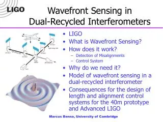
Curvature WFS algorithm One way of doing wavefront sensing is to solve the transport of intensity equation (TIE): Intensity difference between the two defocused images is proportional to the curvature of the wavefront: Iterative FFT method: (C. Roddier and F. Roddier, J Opt Soc Am A10, 2277-87 (1993) ) Make use of the property of Laplacian in Fourier space Iterative algorithm, involves repeatedly setting the boundary condition Orthogonal series expansion: (T. E. Gureyev and K. A. Nugent, J. Opt. Soc. Am. A 13, 1670-1682 (1996)) Non-iterative algorithm, involves integrations over the pupil faster than iterative FFT in general
Further Improving the Accuracy • Both the Iterative FFT and the Series Expansion algorithms are first order approximations valid for highly defocused images. The accuracy can be improved by iteratively compensating the effect of the estimated aberrations on the defocused images. a Create or obtain I1 & I2 b Cocenter I1 & I2 Original intra and extra focal images Iterative FFT or Series Expansion curvature wavefront sensing algorithm to determine initial Westimateor Wresidual c Wavefront compensation to create compensated I1 & I2 d After Wresidualconverges to zero or after a set # of iterations, save (Wcompensated + Wresidual) e Images after compensating the estimated aberrations (2 waves of 45o-astigmatism, in this example)
Algorithmic Challenges for LSST • LSST WFS challenges & algorithmic modifications • Large Central Obscuration (61%) • Fast f/number (f/1.23) • Off-axis Distortion and Vignetting (~1.7o) • Field Dependent Corrections • (covering 1.51° to 1.84°)
Test with Paraxial Lens Model 2 waves of Z4 (defocus) λ=770nm Annular Zernike numbering following Mahajan 1981 Z22=(6,0) Even with annular Zernikes, large obscuration still makes the wavefront harder to recover, because of reduced pixel sampling
What a fast f/# means fp=10.312m image fm=9.427m Large curvature on the principal plane! Red: actual marginal rays Blue: paraxial lens marginal rays
No Aberration? Still non-uniform! Intra Extra When there is no aberration in a fast-beam on-axis system, the intensity distributions on the defocused images are NOT uniform. • If we run our algorithms on a pair of aberration-free images, because of the non-uniform intensity distribution, there will be anormalousfocus+spherical signal. • The obscuration ratio on the pupil plane is different from that on the image plane. (61% vs. 58%) A non-linear mapping from the pupil to the image
Test with LSST On-axis Images 1/2 waves of Z11 (spherical aberration) λ=770nm Annular Zernike numbering following Mahajan 1981 Z22=(6,0)
What Happens at 1.7o Off-axis pupil image ZEMAX view of LSST Field angle (1.185o, 1.185o)
Modeling the Off-axis Distortion Image plane Using paraxial lens model as reference, rayhit coordinate change on the image plane: Aperture @center of wavefrontchip
LSST Off-axis Tests Field angle (1.185o, 1.185o) Single Zernike term: 2λ Z5 (astigmatism 45o) • Vignetting: • Use vignetted pupil mask • Annular Zernikes not orthogonal over pupil • Loss of intensity information on the edge • Effects are observed to be small for most parts of the wavefront chips.
Field-dependent Distortions & Vignetting Intra focal extra focal
Other Field Dependent Corrections • The intra and extra focal images are formed at different field positions • “Migrate” both to the center of wavefront chip using the field-dependent off-axis correction. • Properly normalized the intensities. • Given the split sensor design, the intra focal and extra focal images are vignetted differently • Apply the logical AND of the two pupil masks Vignetting ratio by area (spanning the field angle of the wavefront chips)
Algorithm Performance Beyond Unit Tests • More systematic tests with ZEMAX images • Tests using PhoSimImages • Algorithm Linearity • Covariance Analysis • As part of the LSST Integrated Simulation • Prototype algorithms with real data and real telescopes
LSST Off-axis Tests Field angle (1.185o, 1.185o) Intrinsic aberration 25nm
Split Sensor Tests Original intra Original extra Using the logical AND of the two pupil masks
Tests using PhoSim Images Field=(1.185,1.185) Field=(1.237,1.237) telescope perturbations and atmospheric turbulence turned off Phosim V3.2.6 April 2013
Algorithmic Linearity Z7 on M1M3 (in wave) Z7 on M1M3 (in wave) Wavelength=770nm
Covariance Analysis Total covariance is almost entirely dominated by atmosphere – Diagonal elements (lower left) similar – Singular values (lower right) also similar; some increase for low singular values (Algorithmic + atmospheric) Covariance matrix Variance Singular values
Used in LSST Integrated Simulation With atmosphere, mirror gravity print throughs, polishing errors (M1 only for now), thermal shape errors, and camera internal perturbations
LSST WFS Pipeline Tests on WIYN pODI pODI Full Field (Sep. 13, 2012) LSST wavefront software is open source and is designed for general analysis of intra/extra focal image pairs. • LSST & ODI teams working together to analyze pODI alignment. CCD-4 • Early pODI commissioning tests show wavefront estimation in excellent agreement with obsolete unsupported (but proven) software. Template Blended Pair De-blended Model Fit • De-blending algorithm shown to be effective, maximizing the available sources for wavefront estimation. Early results show excellent agreement with proven software
Conclusions & Future Work • Work has been written up and will be submitted to a journal • Performance analysis has helped with decisions in wavefront sensor design • Code written in MATLAB, and has been converted to Python (Andy Connolly) • Algorithm optimization and code restructuring (Robert Lupton & Mario Juric) • Image pre-processing software has been developed and will be tested and integrated into DM (ISR, source selection, background removal, wavefront image de-blending, etc.) • Algorithm is being used routinely as part of the LSST integrated simulation, where it is being tested with more and more realistic simulated images every day. • Prototype algorithms with real data and real telescopes • DECam– comparing our algorithm with forward modeling algorithm (Aaron Roodman) • WIYN ODI – work in progress (Daniel Harbach) • LBT prime focus – f/1.142 (Mark Wagner) • Magellan – compare curvature measurements with facility SH (Chris Stubbs)