Download
1 / 30
300 likes | 388 Views
Learn about stratification of materials, incomplete block designs, balanced and resolvable block designs, and randomization in agricultural experiments to improve precision and data analysis.

E N D
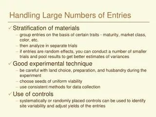
Handling Large Numbers of Entries • Stratification of materials • group entries on the basis of certain traits - maturity, market class, color, etc. • then analyze in separate trials • if entries are random effects, you can conduct a number of smaller trials and pool results to get better estimates of variances • Good experimental technique • be careful with land choice, preparation, and husbandry during the experiment • choose seeds of uniform viability • use consistent methods for data collection • Use of controls • systematically or randomly placed controls can be used to identify site variability and adjust yields of the entries
Incomplete Block Designs • We group into blocks to • Increase precision • Make comparisons under more uniform conditions • But the problem is • As blocks get larger, the conditions become more heterogeneous - precision decreases • So small blocks are preferred, but in a breeding program the number of new selections may be quite large • In other situations, natural groupings of experimental units into blocks may result in fewer units per block than required by the number of treatments (limited number of runs per growth chamber, treatments per animal, etc.)
Incomplete Block Designs • Plots are grouped into blocks that are not large enough to contain all treatments (selections) • Good references: • Kuehl – Chapters 9 and 10 • Cochran and Cox (1957) Experimental Designs
Types of incomplete block designs • Balanced Incomplete Block Designs • each treatment occurs together in the same block with every other treatment an equal number of times - usually once • all pairs are compared with the same precision even though differences between blocks may be large • can balance any number of treatments and any size of block but...treatments and block size fix the number of replications required for balance • often the minimum number of replications required for balance is too large to be practical • Partially balanced incomplete block designs • different treatment pairs occur in the same blocks an unequal number of times or some treatment pairs never occur together in the same block • mean comparisons have differing levels of precision • statistical analysis more complex
Types of incomplete block designs • May have a single blocking criterion • Randomized incomplete blocks • Other designs have two blocking criteria and are based on Latin Squares • Latin Square is a complete block design that requires N=t2. May be impractical for large numbers of treatments. • Row-Column Designs – either rows or columns or both are incomplete blocks • Youden Squares – two or more rows omitted from the Latin Square
Resolvable incomplete block designs • Blocks are grouped so that each group of blocks constitute one complete replication of the treatment • Trials can be managed in the field on a replication-by-replication basis • Field operations can be conducted in stages (planting, weeding, data collection, harvest) • Complete replicates can be lost without losing the whole experiment • If you have two or more complete replications, you can analyze as a RBD if the blocking turns out to be ineffective • Lattice designs are a well-known type of resolvable incomplete block design
Balanced Incomplete Block Designs • t = s*k and b = r*s ≥ t + r - 1 • t = number of treatments • s = number of blocks per replicate • k = number of units per block (block size) • b = total number of blocks in the experiment • r = number of complete replicates • Example • for 16 treatments, 4 blocks/rep, 4 units/block • Need r ≥ 5 • Take home message – with large numbers of treatments, the minimum number of replications required for balance is often too large to be practical
Lattice Designs • Square lattice designs • number of treatments must be a perfect square (t = k2) • blocks per replicate (s) and plots per block (k) are equal (s = k) and are the square root of the number of treatments (t) • for complete balance, number of replicates (r) = k+1 • Rectangular lattice designs • t = s*(s-1) and k = (s-1) • example: 4 x 5 lattice has 4 plots per block, 5 blocks per replicate, and 20 treatments • Alpha lattices • t = s*k • more flexibility in choice of s and k
Randomization • Field Arrangement • blocks composed of plots that are as homogeneous as possible • Randomization Using Basic Plan • randomize order of blocks within replications • randomize the order of treatments within blocks
The Basic Plan for a Square Lattice Block Rep I Rep II Rep III Rep IV 1 1 2 3 1 4 7 1 5 9 1 6 8 2 4 5 6 2 5 8 2 6 7 2 4 9 3 7 8 9 3 6 9 3 4 8 3 5 7 • Balance - each treatment occurs together in the same block with every other treatment an equal number of times (λ = 1)
Example of randomization of a 3 x 3 balanced lattice (t = 9) 1 Assign r random numbers 2 From Basic Plan Random Sequence Rank 372 1 2 217 2 1 963 3 4 404 4 3 Block Rep I Rep II Rep III Rep IV 1 1 2 3 1 4 7 1 5 9 1 6 8 2 4 5 6 2 5 8 2 6 7 2 4 9 3 7 8 9 3 6 9 3 4 8 3 5 7 3 Randomize order of replications 4 Randomize blocks within reps Rep I II III IV 3 2 3 1 2 1 1 3 1 3 2 2 Block Rep I Rep II Rep III Rep IV 1 1 4 7 1 2 3 1 6 8 1 5 9 2 2 5 8 4 5 6 2 4 9 2 6 7 3 3 6 9 7 8 9 3 5 7 3 4 8 5 Resulting new plan Block Rep I Rep II Rep III Rep IV 1 3 6 9 4 5 6 3 5 7 1 5 9 2 2 5 8 1 2 3 1 6 8 3 4 8 3 1 4 7 7 8 9 2 4 9 2 6 7
Partially Balanced Lattices • Simple Lattices • Two replications - use first two from basic plan • 3x3 and 4x4 are no more precise than RBD because error df is too small • Triple Lattices • Three replications - use first three from basic plan • Possible for all squares from 3x3 to 13x13 • Quadruple Lattices • Four replications - use all four • Do not exist for 6x6 and 10x10 - can repeat simple lattice, but analysis is different
Analysis • Details are the same for simple, triple and quadruple • Nomenclature: • yij(l) represents the yield of the j-th treatment in the l-th block of the i-th replication • Two error terms are computed • Eb - Error for block = SSB/r(k-1) • Ee - Experimental error = SSE/((k-1)(rk-k-1))
Computing Sums of Squares • SSTot = S yij(l)2 - (G2/rk2) • SSR = (1/k2) S Rj2 - (G2/rk2) • SSB = (1/kr(r-1)) S Cil2 - (1/k2r(r-1)) S Ci2 • Cil = sum over all replications of yields of all treatments in the l-th block of the i-th replication minus rBil • Bil = sum of yields of the k plots in the l-th block of the i-th replication • Ci = sum of Cil • SST = (1/r) S T2 - (G2/rk2) • SSE = SSTot - SSR - SSB - SST
Adjustment factor • Compare Eb with Ee - If Eb < Ee • then blocks have no effect • analyze as if it were RBD using replications as blocks • If Eb > Ee then compute adjustment factor A • A = (Eb - Ee )/(k(r-1)Eb) • used to compute adjusted yields in data table and table of totals • Compute the effective error mean square • Ee’ = (1+(rkA)/(k+1))Ee • except for small designs (k=3,4), used in t tests and interval estimates
ANOVA Source df SS MS Total rk2-1 SSTOT Rep r-1 SSR Treatments k2-1 SST Block(adj) r(k-1) SSB Eb Intrablock error (k-1)(rk-k-1) SSE Ee
Testing differences • To test significance among adjusted treatment means, compute an adjusted mean square • SSBu = (1/k)SBil2 - (G2/rk2) - SSR • SSTadj = SST- A k (r-1) [ ((rSSBu)/(r-1)(1+kA))-SSB] • Finally, compute the F statistic for testing the differences among the adjusted treatment means • F = (SSTadj / (k2-1))/ Ee • with k2 - 1 degrees of freedom (k-1)(rk-k-1) from MSE
Standard Errors • SE of adjusted treatment mean • = Ee’ / r • SE of difference between adjusted means in same block • = (2Ee/r)(1+(r-1)A) • SE of difference between adjusted means in different blocks • = (2Ee/r)(1+rA) • For larger lattices (k > 4) sufficient to use • = 2Ee’ / r
Relative Precision • Compute the error mean square of a RBD • ERB = ((SSB+SSE)/(k2-1)(r-1)) • Then the relative precision of the lattice is • RP = ERB/Ee’
Rep Blk Yield BilCil Adj I 1 (19) (16) (18) (17) (20) 18.2 13.0 9.5 6.7 10.1 57.5 17.6 1.54 2 (12) (13) (15) (14) (11) 13.3 11.4 14.2 11.9 13.4 64.2 4.2 .37 3 (1) (2) (3) (4) (5) 15.0 12.4 17.3 20.5 13.0 78.2 5.3 .46 4 (22) (24) (21) (25) (23) 7.0 5.9 14.1 19.2 7.8 54.0 -.5 -.04 5 (9) (7) (10) (8) (6) 11.9 15.2 17.2 16.3 16.0 76.6 3.9 .34 Sum 330.5 30.5 2.67 Numerical Example - Simple Lattice
Second Rep Rep Blk Yield BilCil Adj II 1 (23) (18) (3) (8) (13) 7.7 15.2 19.1 15.5 14.7 72.2 -9.9 -.86 2 (5) (20) (10) (15) (25) 15.8 18.0 18.8 14.4 20.0 87.0 -13.3 -1.17 3 (22) (12) (2) (17) (7) 10.2 11.5 17.0 11.0 15.3 65.0 -10.4 -.91 4 (14) (24) (9) (4) (19) 10.9 4.7 10.9 16.6 9.8 52.9 15.5 1.35 5 (6) (16) (11) (21) (1) 20.0 21.1 16.9 10.9 15.0 83.9 -12.4 -1.08 Sum 361.0 -30.5 -2.67 SUM 691.5 0.0 0.00
Unadjusted Yield Totals (1) 30.0 (2) 29.4 (3) 36.4 (4) 37.1 (5) 28.8 (6) 36.0 (7) 30.5 (8) 31.8 (9) 22.8 (10) 36.0 (11) 30.3 (12) 24.8 (13) 26.1 (14) 22.8 (15) 28.6 (16) 34.1 (17) 17.7 (18) 24.7 (19) 28.0 (20) 28.1 (21) 25.0 (22) 17.2 (23) 15.5 (24) 10.6 (25) 39.2 SUM 691.5
ANOVA Source df SS MS Total 49 805.42 Replication 1 18.60 Selection (unadj) 24 621.82 Block in rep (adj) 8 77.59 9.70=Eb Intrablock error 16 87.41 5.46=Ee Eb is greater than Ee so we compute the adjustment factor, A A = (Eb - Ee )/(k(r-1)Eb ) = (9.70 - 5.46)/((5)(1)(9.70)) = 0.0874 Multiply A by the treatment/block sums (C) to get the adjusted totals
Computing Effective Error • Once you have calculated the Adjustment factor (A), calculate the effective mean square (Ee’ ) • Ee’ = (1+(rkA)/(k+1))Ee = (1+(2*5*0.0874)/6)*5.46 = 6.26 • To test significance, compute SSBu • 1/k S Bil2 - Correction factor - SSR • for this example 9834.23-9563.44-18.60=252.18 • Then SST(adj)= • SST – A*k(r-1){ [ r * SSBu/(r-1)(1+kA) ] - SSB} • 621.82-(0.0874)(5)(1) { [ (2 x 252.18)/1 * (1+5*0.0874)]-77.59} = 502.35
Test Statistics • FT to test differences among the adjusted treatment means: • (SST(adj)/(k2-1))/Ee’ • (502.35/24)/6.26 = 3.34 • Standard Error of a selection mean • = Ee’/r = 6.26/2 = 1.77 • LSI can be computed since k > 4 • ta 2Ee’/r = 1.746 (2x6.26)/2 = 4.37
Relative precision • How does the precision of the Lattice compare to that of a randomized block design? • First compute MSE for the RBD as: ERB = (SSB+SSE)/(k2 - 1)(r -1) = (77.59 + 87.41)/(24)(1) = 6.88 • Then % relative precision = • (ERB / Ee’ )100 = (6.88/6.26)*100 = 110.0%
Report of Statistical Analysis • Because of variation in the experimental site and because of economic considerations, a 5x5 simple lattice design was used • LSI at the 5% level was 4.37 • Five new selections outyielded the long term check (12.80kg/plot) • One new selection (4) with a yield of 19.46 significantly outyielded the local check (1) • None of the new selections outyielded the late release whose mean yield was 19.00 • Use of the simple lattice resulted in a 10% increase in precision when compared to a RBD
Cyclic designs • Incomplete Block Designs discussed so far require extensive tables of design plans. Must be careful not to make mistakes when assigning treatments to experimental units and during field operations • Cyclic designs are a type of incomplete block design that are relatively easy to construct and implement
Alpha designs • Patterson and Williams, 1976 • Described a way to construct incomplete block designs for any number of treatments (t) and block size (k), such that t is a multiple of k. Includes (0,1)-lattice designs. • α-designs are available for many (r,k,s) combinations • r is the number of replicates • k is the block size • s is the number of blocks per replicate • number of treatments t = ks • Efficient α-designs exist for some combinations for which conventional lattices do not exist • Can accommodate unequal block sizes
Alpha designs • Design Software • The current version of Gendex can generate designs with up to 10,000 entries • http://www.designcomputing.net/gendex/ • Evaluation copy is free • Cost for perpetual/personal license is $199 • Others: Alpha+, CycDesigN • Analysis can be done with SAS