Download
1 / 20
200 likes | 234 Views
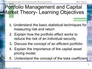
Portfolio Management and Capital Market Theory- Learning Objectives. 1. Understand the basic statistical techniques for measuring risk and return 2. Explain how the portfolio effect works to reduce the risk of an individual security. 3. Discuss the concept of an efficient portfolio

E N D
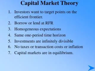
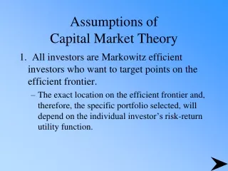
Portfolio Management and Capital Market Theory- Learning Objectives 1.Understand the basic statistical techniques for measuring risk and return 2. Explain how the portfolio effect works to reduce the risk of an individual security. 3. Discuss the concept of an efficient portfolio 4. Explain the importance of the capital asset pricing model. 5. Understand the concept of the beta coefficient
Investment j Standard Deviation= Note that the average is the same for each investment but that the standard deviation is different. Also note that this model assumes no correlation between i and j. Investment i Standard Deviation=
Portfolio Effect ( 2 stocks, equal weight) Portfolio Return k Assume stocks x1 and x2 with parameters: x1 = .5 K1 = 10% s1 = 3.9 x2 = .5 K2 = 10% s2 = 5.1 Definition of portfolio expected return according to equation 21-3. Kp = x1 K1 + x2 K2 = .5(10 %) + .5(10 %) = 10%
i = .52(3.9)2+.52(5.1)2+2(.5)(.5) rij (3.9)(5.1) Standard Deviation of a Two-Stock Portfolio( 2 stocks, equal weight) = 3.85 +6.4 + .5 rij 19.9 rijsp +1.0 4.5 p + .5 3.9 0.0 3.2 - .5 2.3 - .7 1.8 -1.0 0.0 Calculated standard deviation with differing correlation coefficients. Correlation Coefficient
Developing and Efficient Portfolio • Many possible portfolios (i.e., combinations of investments) • The investor determines his personal risk-return criteria • An investor should select from the most efficient portfolios (i.e., those with the maximum return for a given risk). • Portfolios do not exist above the "efficient frontier"
15 14 13 12 11 10 9 0 1 2 3 4 5 6 8 7 Diagram of Risk-Return Trade-Offs Expected return Kp (Figure 21-3) H F G E D C Efficientfrontier A B Portfolio standard deviation (p) (risk)
15 14 13 12 Inefficient portfolios 11 10 9 0 1 2 3 4 5 6 8 7 Diagram of Risk-Return Trade-offs Expected return Kp H F G E D C Efficientfrontier A B Portfolio standard deviation (p) (risk)
Capital Asset Pricing Model • The CAPM introduces the risk-free asset where RF = 0. • Under the CAPM, investors combine the risk-free asset with risky portfolios on the efficient frontier.
The CAPM and Indifference Curves Maximum attainable risk-return (Fig21-8) Z Expected return Kp Initial: risk free point M Satisfies efficient frontier Efficientfrontier RF Risk Return line Portfolio standard deviation (p)
Capital Asset Pricing Model • The RFMZ line represents investment opportunities that are superior to the existing efficient frontier. • RFMZ line is called capital market line. • How do investors reach points on the RFMZ line?
Capital Asset Pricing Model • To attain line RFM • Buy a combination of RFF and M portfolio • To attain M Z • Buy M portfolio and borrow additional funds at the risk-free rate.
Capital Asset Pricing Model • Portfolio M is an optimum “market basket of investments.” • M portfolio can be represented by NYSE,or S&P 500. • Broadly based index is better than narrowly based index.
Security Market Line • Refers to an individual stock • Trade-off between risk & return • Analogous to Capital Market Line for market portfolios • Formula is: • Ki = RF + bi (KM - RF)
Illustration of the Capital Market Line return (Figure 21-12) Expected return Kp KM Security Market Line (CML) RF Market standard deviation O 2.0 1.0 Risk (Beta)
Sharpe measure Total portfolio return - Risk-free rate Portfolio standard deviation = .12 - .05 .14 Sharpe Measure = = 0.50 Sharpe Approach Market data: KF = 5% Portfolio Data: kp = .12 bp = 1.2 sp = .14 Measures excess return per unit of total risk. Also known as "excess return to variability" ratio. Higher values indicate superior performance
Treynor measure Total portfolio return - Risk-free rate Portfolio Beta = .10 - .06 0.9 Treynor Measure = = 0.044 Treynor Approach Market data: KF = 6% Portfolio Data: kp = 0.10 bp = 0.9 Measures excess return per unit of systematic risk. Also known as "excess return to volatility" ratio. Higher values indicate superior performance
Jensen Approach • Alpha (average differential) return indicates the difference between a) the return on the fund and b) a point on the market line that corresponds to a beta equal that of the fund. • Alpha = the actual rate of return minus the rate of return predicted by the CAPM. • The McGraw-Hill Companies, Inc.,1999
Market line 6 5 4 3 2 1 -1 -2 -3 1.5 O .5 1.O Figure 22-2 Risk-Adjusted Portfolio Returns ML = a + b (EMR) EMR is "excess market return" Excess returns (%) MarketM Z Y O Portfolio Beta
Jensen Approach • Jensen computed the alpha value of 115 mutual funds. • The average alpha was a negative 1.1% and only 39 out of 115 funds had a positive alpha.