Download
1 / 27
300 likes | 610 Views
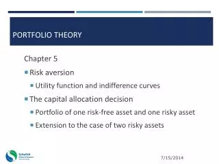
Portfolio Theory. Chapter 5 Risk aversion Utility function and indifference curves The capital allocation decision Portfolio of one risk-free asset and one risky asset Extension to the case of two risky assets. p = 0.6. W 1 = 150; Profit = 50. 1-p = 0.4. W 2 = 80; Profit = -20.

E N D
Portfolio Theory Chapter 5 • Risk aversion • Utility function and indifference curves • The capital allocation decision • Portfolio of one risk-free asset and one risky asset • Extension to the case of two risky assets
p = 0.6 W1 = 150; Profit = 50 1-p = 0.4 W2 = 80; Profit = -20 Example of a Risky Investment W = 100 E(r) = pr1 + (1-p)r2 = ? 2 = p[r1 – E(r)]2 + (1-p) [r2 – E(r)]2 = ?
p = 0.6 W1 = 150 Profit = 50 Risky Investment W2= 80 Profit = -20 1-p = .4 Risk Free T-bills Profit = 5 Expanding the choice set 100 Risk Premium = 22% - 5% = 17%
Risk Preference/Attitude/Tolerance • Investor’s view of risk • Risk Averse • Risk Neutral • Risk Seeking / loving • Utility Function • Private value, in our case, of risk and return • Example: One popular utility function used in investments is U = E ( r ) – 0.5 A s2 • “A” measures the degree of risk aversion
Risky Investment Example U = E ( r ) - 0.5 A s2 = 0.22 - 0.5 A (0.34) 2 Risk AversionAUtility High 5 - 0.07 3 0.05 Low 1 0.16 Compared to utility of T-bill = 0.05
Indifference curves • U = E ( r ) - 0.5 A s2 Three variables on a 2-dimensional diagram Links portfolios that yield the same level of utility
Indifference curve example • All four portfolios yield the same level of utility (U = 0.02) • Hence, they would lie on the same indifference curve in the diagram
E(rp) Increasing Utility P Indifference Curves
The capital allocation decision • Task: allocate capital (funds) between risky and risk-free assets • Examine risk/return tradeoff • If financial market is efficient, no free lunch plan • Demonstrate how different degrees of risk aversion will affect allocations between risky and risk-free assets
Portfolio Mathematics • The rate of return of a portfolio is a weighted average of the return of each asset in the portfolio, with the portfolio proportions as weights • Consider a two-asset case: rp = w1r1 + w2r2 • Example of weights: (0.5, 0.5), (0.4, 0.6), (0.3, 0.7)
Portfolio Mathematics • Mean return of a portfolio E(rp) = w1E(r1)+ w2E(r2) • Variance of portfolio (proxy for risk) • When two assets with variances, 12 and 22 , are combined into a portfolio with portfolio weights w1 and w2, respectively, the portfolio variance is: • What if one of the assets is risk-free?
Portfolio of one risky asset and one risk-free asset • Risky portfolio P: E(rp) = 15% and p = 22% • Risk-free asset: rf= 7% and rf = 0% • And the proportions invested: y in P and (1-y) in F
E(rc) = yE(rp) + (1 - y)rf = rf + y[E(rp) – rf] where rc = “combined” portfolio return If, for example, y = .75 E(rc) = .75(.15) + .25(.07) = .13 or 13% Expected return of the “combined” portfolio
Standard Deviation of the combined portfolio • Recall that the variance is: • Apply to the current example: • This collapses to the following standard deviation:
Standard deviation of combined portfolio • If y = 0.75, then c = 0.75(0.22) = 0.165 or 16.5% • If y = 1, then c = 1(0.22) = 0.22 or 22% • If y = 0, then c = 0(0.22) = 0%
The Investment Opportunity Set with a Risky Asset and a Risk-Free Asset (CAL)
Algebraically.... (in order to be exact) • Maximize U = E(rc) – 0.5Ac2 with respect to y • Substitute in E(rc) and c2 • The solution is: • Numerical example:
y* = 0.41 • Given this optimal weight, what is • the portfolio mean? E(rC) = 0.41 x 0.15 + (1 – 0.41) x 0.07 = 0.1028 or 10.28% • and the portfolio standard deviation? C= 0.41 x 0.22 = 0.0902 or 9.02%
Indifference Curves for U = .05 and U = .09 with A = 2 and A = 4
Leveraged portfolios • Extend beyond y = 1 • Borrow at the risk-free rate and invest in more than 100% of the portfolio in the risky asset • Can think of as short selling the risk-free asset • Using 50% leverage: E(rc) = (-0.5) (0.07) + (1.5) (0.15) = .19 c = (1.5) (0.22) = .33
E(r) P Borrower 7% Lender p= 22% CAL with Risk Preferences
An Application of the CAL • Client likes the fund, but not like the volatility (of the returns) • In this case, manager may let the client choose the level of volatility • If client wants a higher level of volatility, use leverage • If client wants a lower level of volatility, put a portion in cash • Slide up or down the CAL
The Opportunity Set with Differential Borrowing and Lending Rates