Download
1 / 57
800 likes | 2.44k Views
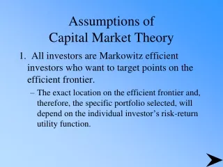
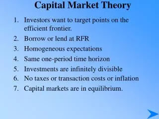
Capital Market Theory. Investors want to target points on the efficient frontier. Borrow or lend at RFR Homogeneous expectations Same one-period time horizon Investments are infinitely divisible No taxes or transaction costs or inflation Capital markets are in equilibrium.

E N D
Capital Market Theory • Investors want to target points on the efficient frontier. • Borrow or lend at RFR • Homogeneous expectations • Same one-period time horizon • Investments are infinitely divisible • No taxes or transaction costs or inflation • Capital markets are in equilibrium.
Assumptions of Capital Market Theory • Some of these assumptions are unrealistic • Relaxing many of these assumptions would have only minor influence on the model and would not change its main implications or conclusions. • A theory should be judged on how well it explains and helps predict behavior, not on its assumptions.
Risk-Free Asset • An asset with zero standard deviation • Zero correlation with all other risky assets • Provides the risk-free rate of return (RFR) • Will lie on the vertical axis of a portfolio graph
Covariance with a Risk-Free Asset Covariance between two sets of returns is Because the returns for the risk free asset are certain, Thus Ri = E(Ri), and Ri - E(Ri) = 0 Consequently, the covariance of the risk-free asset with any risky asset or portfolio will always equal zero. Similarly the correlation between any risky asset and the risk-free asset would be zero.
Combining a Risk-Free Asset with a Risky Portfolio Expected return the weighted average of the two returns This is a linear relationship
Combining a Risk-Free Asset with a Risky Portfolio Standard deviation The expected variance for a two-asset portfolio is Substituting the risk-free asset for Security 1, and the risky asset for Security 2, this formula would become Since we know that the variance of the risk-free asset is zero and the correlation between the risk-free asset and any risky asset i is zero we can adjust the formula
Combining a Risk-Free Asset with a Risky Portfolio Given the variance formula the standard deviation is Therefore, the standard deviation of a portfolio that combines the risk-free asset with risky assets is the linear proportion of the standard deviation of the risky asset portfolio.
Combining a Risk-Free Asset with a Risky Portfolio Since both the expected return and the standard deviation of return for such a portfolio are linear combinations, a graph of possible portfolio returns and risks looks like a straight line between the two assets.
Portfolio Possibilities Combining the Risk-Free Asset and Risky Portfolios on the Efficient Frontier Exhibit 8.1 D M C B A RFR
Risk-Return Possibilities with Leverage To attain a higher expected return than is available at point M (in exchange for accepting higher risk) • Either invest along the efficient frontier beyond point M, such as point D • Or, add leverage to the portfolio by borrowing money at the risk-free rate and investing in the risky portfolio at point M
Portfolio Possibilities Combining the Risk-Free Asset and Risky Portfolios on the Efficient Frontier CML Borrowing Lending Exhibit 8.2 M RFR
The Market Portfolio • Because portfolio M lies at the point of tangency, it has the highest portfolio possibility line • Everybody will want to invest in Portfolio M and borrow or lend to be somewhere on the CML • Therefore this portfolio must include ALL RISKY ASSETS
The Market Portfolio Because the market is in equilibrium, all assets are included in this portfolio in proportion to their market value
The Market Portfolio Because it contains all risky assets, it is a completely diversified portfolio, which means that all the unique risk of individual assets (unsystematic risk) is diversified away
Systematic Risk • Only systematic risk remains in the market portfolio • Systematic risk is the variability in all risky assets caused by macroeconomic variables • Systematic risk can be measured by the standard deviation of returns of the market portfolio and can change over time
Examples of Macroeconomic Factors Affecting Systematic Risk • Variability in growth of money supply • Interest rate volatility • Variability in • industrial production • corporate earnings • cash flow
How to Measure Diversification • All portfolios on the CML are perfectly positively correlated with each other and with the completely diversified market Portfolio M • A completely diversified portfolio would have a correlation with the market portfolio of +1.00
Diversification and the Elimination of Unsystematic Risk • The purpose of diversification is to reduce the standard deviation of the total portfolio • This assumes that imperfect correlations exist among securities • As you add securities, you expect the average covariance for the portfolio to decline • How many securities must you add to obtain a completely diversified portfolio?
Diversification and the Elimination of Unsystematic Risk Observe what happens as you increase the sample size of the portfolio by adding securities that have some positive correlation
Number of Stocks in a Portfolio and the Standard Deviation of Portfolio Return Standard Deviation of Return Exhibit 8.3 Unsystematic (diversifiable) Risk Total Risk Standard Deviation of the Market Portfolio (systematic risk) Systematic Risk Number of Stocks in the Portfolio
The CML and the Separation Theorem • The CML leads all investors to invest in the M portfolio • Individual investors should differ in position on the CML depending on risk preferences • How an investor gets to a point on the CML is based on financing decisions • Risk averse investors will lend part of the portfolio at the risk-free rate and invest the remainder in the market portfolio
The CML and the Separation Theorem Investors preferring more risk might borrow funds at the RFR and invest everything in the market portfolio
The CML and the Separation Theorem The decision of both investors is to invest in portfolio M along the CML (the investment decision) CML B M A PFR
The CML and the Separation Theorem The decision to borrow or lend to obtain a point on the CML is a separate decision based on risk preferences (financing decision)
The CML and the Separation Theorem Tobin refers to this separation of the investment decision from the financing decision, the separation theorem
A Risk Measure for the CML • Covariance with the M portfolio is the systematic risk of an asset • The Markowitz portfolio model considers the average covariance with all other assets in the portfolio • The only relevant portfolio is the M portfolio
A Risk Measure for the CML Together, this means the only important consideration is the asset’s covariance with the market portfolio
A Risk Measure for the CML Because all individual risky assets are part of the M portfolio, an asset’s rate of return in relation to the return for the M portfolio may be described using the following linear model: where: Rit = return for asset i during period t ai = constant term for asset i bi = slope coefficient for asset i RMt = return for the M portfolio during period t = random error term
The Capital Asset Pricing Model: Expected Return and Risk • The existence of a risk-free asset resulted in deriving a capital market line (CML) that became the relevant frontier • An asset’s covariance with the market portfolio is the relevant risk measure • This can be used to determine an appropriate expected rate of return on a risky asset - the capital asset pricing model (CAPM)
The Capital Asset Pricing Model: Expected Return and Risk • CAPM indicates what should be the expected or required rates of return on risky assets • This helps to value an asset by providing an appropriate discount rate to use in dividend valuation models • You can compare an estimated rate of return to the required rate of return implied by CAPM - over/under valued ?
The Security Market Line (SML) • The relevant risk measure for an individual risky asset is its covariance with the market portfolio (Covi,m) • This is shown as the risk measure • The return for the market portfolio should be consistent with its own risk, which is the covariance of the market with itself - or its variance:
Exhibit 8.5 Graph of Security Market Line (SML) SML RFR
The Security Market Line (SML) The equation for the risk-return line is We then define as beta
Exhibit 8.6 Graph of SML with Normalized Systematic Risk SML Negative Beta RFR
Determining the Expected Rate of Return for a Risky Asset • The expected rate of return of a risk asset is determined by the RFR plus a risk premium for the individual asset • The risk premium is determined by the systematic risk of the asset (beta) and the prevailing market risk premium (RM-RFR)
Determining the Expected Rate of Return for a Risky Asset Assume: RFR = 5% (0.05) RM = 9% (0.09) Implied market risk premium = 4% (0.04) E(RA) = 0.05 + 0.70 (0.09-0.05) = 0.078 = 7.8% E(RB) = 0.05 + 1.00 (0.09-0.05) = 0.090 = 09.0% E(RC) = 0.05 + 1.15 (0.09-0.05) = 0.096 = 09.6% E(RD) = 0.05 + 1.40 (0.09-0.05) = 0.106 = 10.6% E(RE) = 0.05 + -0.30 (0.09-0.05) = 0.038 = 03.8%
Determining the Expected Rate of Return for a Risky Asset • In equilibrium, all assets and all portfolios of assets should plot on the SML • Any security with an estimated return that plots above the SML is underpriced • Any security with an estimated return that plots below the SML is overpriced • A superior investor must derive value estimates for assets that are consistently superior to the consensus market evaluation to earn better risk-adjusted rates of return than the average investor
Identifying Undervalued and Overvalued Assets • Compare the required rate of return to the expected rate of return for a specific risky asset using the SML over a specific investment horizon to determine if it is an appropriate investment • Independent estimates of return for the securities provide price and dividend outlooks
Calculating Systematic Risk: The Characteristic Line The systematic risk input of an individual asset is derived from a regression model, referred to as the asset’s characteristic line with the model portfolio: where: Ri,t = the rate of return for asset i during period t RM,t = the rate of return for the market portfolio M during t
The Impact of the Time Interval • Number of observations and time interval used in regression vary • Value Line Investment Services (VL) uses weekly rates of return over five years • Merrill Lynch, Pierce, Fenner & Smith (ML) uses monthly return over five years • There is no “correct” interval for analysis • Weak relationship between VL & ML betas due to difference in intervals used • The return time interval makes a difference, and its impact increases as the firm’s size declines
The Effect of the Market Proxy • The market portfolio of all risky assets must be represented in computing an asset’s characteristic line • Standard & Poor’s 500 Composite Index is most often used • Large proportion of the total market value of U.S. stocks • Value weighted series
Weaknesses of Using S&P 500as the Market Proxy • Includes only U.S. stocks • The theoretical market portfolio should include U.S. and non-U.S. stocks and bonds, real estate, coins, stamps, art, antiques, and any other marketable risky asset from around the world
Differential Borrowing and Lending Rates Heterogeneous Expectations and Planning Periods Zero Beta Model does not require a risk-free asset Transaction Costs with transactions costs, the SML will be a band of securities, rather than a straight line Relaxing the Assumptions
Heterogeneous Expectations and Planning Periods will have an impact on the CML and SML Taxes could cause major differences in the CML and SML among investors Relaxing the Assumptions
Stability of Beta betas for individual stocks are not stable, but portfolio betas are reasonably stable. Further, the larger the portfolio of stocks and longer the period, the more stable the beta of the portfolio Comparability of Published Estimates of Beta differences exist. Hence, consider the return interval used and the firm’s relative size Empirical Tests of the CAPM
Effect of Skewness on Relationship investors prefer stocks with high positive skewness that provide an opportunity for very large returns Effect of Size, P/E, and Leverage size, and P/E have an inverse impact on returns after considering the CAPM. Financial Leverage also helps explain cross-section of returns Relationship Between Systematic Risk and Return
Effect of Book-to-Market Value Fama and French questioned the relationship between returns and beta in their seminal 1992 study. They found the BV/MV ratio to be a key determinant of returns Summary of CAPM Risk-Return Empirical Results the relationship between beta and rates of return is a moot point Relationship Between Systematic Risk and Return
There is a controversy over the market portfolio. Hence, proxies are used There is no unanimity about which proxy to use An incorrect market proxy will affect both the beta risk measures and the position and slope of the SML that is used to evaluate portfolio performance The Market Portfolio: Theory versus Practice
Summary • The assumption of capital market theory expand on those of the Markowitz portfolio model and include consideration of the risk-free rate of return