Download
1 / 52
530 likes | 988 Views
Thermodynamics and Phase Diagrams from Cluster Expansions . Dane Morgan University of Wisconsin, ddmorgan@wisc.edu SUMMER SCHOOL ON COMPUTATIONAL MATERIALS SCIENCE Hands-on introduction to Electronic Structure and Thermodynamics Calculations of Real Materials

E N D
Thermodynamics and Phase Diagrams from Cluster Expansions Dane Morgan University of Wisconsin, ddmorgan@wisc.edu SUMMER SCHOOL ON COMPUTATIONAL MATERIALS SCIENCE Hands-on introduction to Electronic Structure and Thermodynamics Calculations of Real Materials University of Illinois at Urbana-Champaign, June 13-23, 2005
The Cluster Expansion and Phase Diagrams Cluster Expansion a = cluster functions s = atomic configuration on a lattice H. Okamoto, J. Phase Equilibria,'93 How do we get the phase diagram from the cluster expansion Hamiltonian?
Outline • Phase Diagram Basics • Stable Phases from Cluster Expansion - the Ground State Problem • Analytical methods • Optimization (Monte Carlo, genetic algorithm) • Exhaustive search • Phase Diagrams from Cluster Expansion: Semi-Analytical Approximations • Low-T expansion • High-T expansion • Cluster variation method • Phase Diagrams from Cluster Expansion: Simulation with Monte Carlo • Monte Carlo method basics • Covergence issues • Determining phase diagrams without free energies. • Determining phase diagrams with free energies.
What is A Phase Diagram? • Phase: A chemically and structurally homogeneous portion of material, generally described by a distinct value of some parameters (‘order parameters’). E.g., ordered L10 phase and disordered solid solution of Cu-Au • Gibb’s phase rule for fixed pressure: • F(degrees of freedom) = C(# components) - P(# phases) + 1 • Can have 1 or more phases stable at different compositions for different temperatures • For a binary alloy (C=2) can have 3 phases with no degrees of freedom (fixed composition and temperature), and 2 phases with 1 degree of freedom (range of temperatures). • The stable phases at each temperature and composition are summarized in a phase diagram made up of boundaries between single and multiple phase regions. Multi-phase regions imply separation to the boundaries in proportions consistent with conserving overall composition. 3 phase 1 phase 2 phase H. Okamoto, J. Phase Equilibria,'93 The stable phases can be derived from optimization of an appropriate thermodynamic potential.
Thermodynamics of Phase Stability • The stable phases minimize the total thermodynamic potential of the system • The thermodynamic potential for a phase a of an alloy under atmospheric pressure: • The total thermodynamic potential is • The challenges: • What phases d might be present? • How do we get the Fd from the cluster expansion? • How use Fd to get the phase diagram? • Note: Focus on binary systems (can be generalized but details get complex), focus on single parent lattice (multiple lattices can be treated each separately)
Stable Phases from Cluster Expansion –the Ground State Problem
Determining Possible Phases • Assume that the phases that might appear in phase diagram are ground states (stable phases at T=0). This could miss some phases that are stabilized by entropy at T>0. • T=0 simplifies the problem since T=0 F is given by the cluster expansion directly. Phases d are now simply distinguished by different fixed orderings sd. • So we need only find the s that give the T=0 stable states. These are the states on the convex hull. H. Okamoto, J. Phase Equilibria,'93
The Convex Hull • None of the red points give the lowest F=SFd. Blue points/lines give the lowest energy phases/phase mixtures. • Constructing the convex hull given a moderate set of points is straightforward (Skiena '97) • But the number of points (structures) is infinite! So how do we get the convex hull? Energy A B CB a d b 2-phase region Convex Hull in blue 1-phase point
Getting the Convex Hull of a Cluster Expansion Hamiltonian • Linear programming methods • Elegantly reduce infinite discrete problem to finite linear continuous problem. • Give sets of Lattice Averaged (LA) cluster functions {LA(f)} of all possible ground states through robust numerical methods. • But can also generate many “inconstructable” sets of {LA(f)} and avoiding those grows exponentially difficult. • Optimized searching • Search configuration space in a biased manner to minimize the energy (Monte Carlo, genetic algorithms). • Can find larger unit cell structures that brute force searching • Not exhaustive – can be difficult to find optimum and can miss hard to find structures, even with small unit cells. • Brute force searching • Enumerate all structures with unit cells < Nmax atoms and build convex hull from that list. • Likely to capture most reasonably small unit cells (and these account for most of what are seen in nature). • Not exhaustive – can miss larger unit cell structures. (Blum and Zunger, Phys. Rev. B, ’04) (Zunger, et al., http://www.sst.nrel.gov/topics/new_mat.html)
Phase Diagrams from Cluster Expansion: Semi-Analytical Approximations
Semi-Analytic Expressions for F (F) From basic thermodynamics we can write F in terms of the cluster expansion Hamiltonian • High-temperature expansion • Low-temperature expansion • Mean-field theory Cluster expansion For a binary alloy on a fixed lattice the number of particles is conserved since NA+NB=N=# sites, thus we can write the semi-grand canonical potentialF in terms of one chemical potential and NB (Grand canonical = particle numbers can change, Semi-Grand canonical = particle types can change but overall number is fixed) But this is an infinite summation – how can we evaluate F?
High-Temperature Expansion Assume x=b(E-mn) is a small number (high temperature) and expand the ln(exp(-x)) Could go out to many higher orders …
High-Temperature Expansion Example (NN Cluster Expansion) z = # NN per atom So first correction is second order in bVNN and reduces the free energy
Low-Temperature Expansion Start in a known ground state a, with chemical potentials that stabilize a, and assume only lowest excitations contribute to F This term assumed small Expand ln in small term Keep contribution from single spin flip at a site s
Low-Temperature Expansion Example(NN Cluster Expansion) Assume an unfrustrated ordered phase at c=1/2 So first correction goes as exp(-2zbVNN) and reduces the free energy
Transition Temperature from LT and HT Expansion NN cluster expansion on a simple cubic lattice (z=6) VNN>0 antiferromagnetic ordering kBTc kBTc/|zV|=0.721 (0th), 0.688 (1st), 0.7522 (best known)
Mean-Field Theory – The Idea The general idea: Break up the system into small clusters in an average “bath” that is not treated explicitly For a small finite lattice with N-sites finding f is not hard – just sum 2N terms Treated fully For an infinite lattice just treat subclusters explicitly with mean field as boundary condition Mean field
Implementing Mean-Field TheoryThe Cluster Variation Method (Kikuchi, Phys. Rev. '51) • Write thermodynamic potential F in terms of probabilities of each configuration r(s), F[{r(s)}]. • The true probabilities and equilibrium F are given by minimizing F[{r(s)}] with respect to {r(s)}, ie, dF[{r(s)}]/d{r(s)}=0. • Simplify r(s) using mean-field ideas to depend on only a few variables to make solving dF[{r(s)}]/d{r(s)}=0 tractable.
Writing f[{r(s)}]. Where
Factoring the Probability to Simplify r(s) Has 2N values Has 2NhM values – much smaller Cluster of lattice points. Maximal size cluster of lattice points to treat explicitly. Irreducible probabilities. Depend on only spin values in cluster of points h. Have value 1 if the sites in h are uncorrelated (even if subclusters are correlated) Probability of finding spins sh on cluster of sites h. Kikuchi-Barker coefficients
Truncating the Probability Factorization = Mean Field Treated fully Mean field Setting treats each cluster aM explicitly and embeds it in the appropriate average environment aM
The Mean-Field Potential F now depends on only and can be minimized to get approximate probabilities and potential
The Modern Formalism • Using probabilities as variables is hard because you must • Maintain normalization (sums = 1) • Maintain positive values • Include symmetry • A useful change of variables is to write probabilities in terms of correlation functions – this is just a cluster expansion of the probabilities
The CVM Potential d D a Degeneracies (multiplicities) Kikuchi-Barker coefficients The phase Clusters of sites a,b t Cluster functions for each cluster – associated with multiple species m Number of species {aM} Set of possible maximal clusters Orbit of clusters under symmetry operations of phase d Od V V matrix that maps correlation functions to probabilities x Correlation function (thermally averaged cluster functions) For a multicomponent alloy
Simplest CVM Approximation – The Point(Bragg-Williams, Weiss Molecular Field) aM=Single point on lattice For a disorderd phase on a lattice with one type of site
CVM Point Approximation - Bragg-Williams(NN Cluster Expansion) Disordered phase – more complex for ordered phases
Bragg-Williams Approximation (NN Cluster Expansion) Predicts 2-phase behavior Critical temperature Single phase behavior
Comparison of Bragg-Williams and High-Temperature Expansion Assume High-temperature Bragg-Williams Optimize F over cB to get lowest value cB=1/2 Bragg-Williams has first term of the high-temperature expansion, but not second. Second term is due to correlations between sites, which is excluded in BW (point CVM)
Critical Temperatures HT/LT approx: kBTc/|zV|=0.721 (0th), 0.688 (1st) de Fontaine, Solid State Physics‘79
Limitations of the CVM (Mean-Field), High- and Low-Temperature Expansions • CVM • Inexact at critical temperature, but can be quite accurate. • Number of variable to optimize over (independent probabilities within the maximal cluster) grows exponentially with maximal cluster size. • Errors occur when Hamiltonian is longer range than CVM approximation – want large interactions within the maximal cluster. • Modern cluster expansions use many neighbors and multisite clusters that can be quite long range. • CVM not applicable for most modern long-range cluster expansions. Must use more flexible approach – MonteCarlo! • High- and Low-Temperature Expansions • Computationally quite complex with many terms • Many term expansions exist but only for simple Hamiltonians • Again, complex long-range Hamiltonians and computational complexity requires other methods – Monte Carlo!
Phase Diagrams from Cluster Expansion: Simulation with Monte Carlo
What Is MC and What is it for? • MC explores the states of a system stochastically with probabilities that match those expected physically • Stochastic means involving or containing a random variable or variables, which is practice means that the method does things based on values of random numbers • MC is used to get thermodynamic averages, thermodynamic potentials (from the averages), and study phase transitions • MC has many other applications outside materials science, where is covers a large range of methods using random numbers • Invented to study the neutron diffusion in bomb research at end of WWII • Called Monte Carlo since that is where gambling happens – lots of chance! http://www.monte-carlo.mc/principalitymonaco/index.html http://www.monte-carlo.mc/principalitymonaco/entertainment/casino.html
MC Sampling • Can we perform this summation numerically? • Simple Monte Carlo Sampling: Choose states s at random and perform the above summation. Need to get Z, but can also do this by sampling at random • This is impractically slow because you sample too many terms that are near zero r(s) is the probability of a having configuration s
Problem with Simple MC Samplingr(s) is Very Sharply Peaked Almost all the contribution to an integral over r(s) comes from here r(s) Sampling states here contributes ≈0 to integral States s E.g., Consider a non-interacting cluster expansion spin model with H=-mNB. For b=m=1 cB=1/(1+e)=0.27. For N=1000 sites the probability of a configuration with cB=0.5 compared to cB=0.27 is P(cB=0.5)/P(CB=0.27)=exp(-NDcB)=10-100
Better MC Sampling • We need an algorithm that naturally samples states for which r(s) is large. Ideally, we will choose states with exactly probability r(s) because • When r(s) is small (large), those s will not (will) be sampled • In fact, if we choose states with probability r(s), then we can write the thermodynamic average as • r(s) is the true equilibrium thermodynamic distribution, so our sampling will generate states that match those seen in an equilibrium system, which make them easy to interpret • The way to sample with the correct r(s) is called the Metropolis algorithm
Detailed Balance and The Metropolis Algorithm • We wants states to occur with probability r(s) in the equilibrated simulation and we want to enforce that by how we choose new states at each step (how we transition). • Impose detailed balance condition (at equilibrium the flux between two states is equal) so that equilibrium probabilities will be stable r(o)p(o→n)=r(n)p(n→o) • Transition matrix p(o→n) = a(o→n) x acc(o→n), where a is the attempt matrix and acc is the acceptance matrix. • Choose a(o→n) symmetric (just pick states uniformly): a(o→n)=a(n→o) • Then r(o)p(o→n)=r(n)p(n→o) r(o)xacc(o→n)=r(n)xacc(n→o) acc(o→n)/acc(n→o) = r(n)/r(o) = exp(-bF(n))/exp(-bF(o)) • So choose acc(o→n) = r(n)/r(o) if r(n)<r(o) 1 if r(n)>=r(o) This keeps detailed balance (stabilizes the probabilities r(s)) and equilibrates the system if it is out of equilibrium – this is the Metropolis Algorithm There are other solutions but this is the most commonly used
The Metropolis Algorithm (General) • An algorithm to pick a series of configurations so that they asymptotically appear with probability r(s)=exp(-bE(s)) • Assume we are in state si • Choose a new state s*, and define DE=E(s*)-E(s) • If DE<0 then accept s* • If DE>0 then accept s* with probability exp(-bDE) • If we accept s* then increment i, set si=s* and return to 1. in a new state • If we reject s* then return to 1. in the same state state si • This is a Markov process, which means that the next state depends only on the previous one and none before.
Metropolis Algorithm for Cluster Expansion Model (Real Space) • We only need to consider spin states • Assume the spins have value (s1 ,… sj ,…, sN) • Choose a new set of spins by flipping, sj* = -sj, where i is chosen at random • Find DF=E(s1 ,… -sj ,…, sN)-E(s1 ,… sj,…, sN)-msj (note that this can be done quickly be only recalculating the energy contribution of spin i and its neighbors) • If DF<0 then accept spin flip • If DF>0 then accept spin flipwith probability exp(-bDF) • If we reject spin flipthen change nothing and return to 1 • The probability of seeing any set of spins s will tend asymptotically to
Obtaining Thermal Averages From MC • The MC algorithm will converge to sample states with probability r(s). So a thermal average is given by • Note that Nmcs should be taken after the system equilibrates • Fluctuations are also just thermal averages and calculated the same way
Energy Vs. MC Step Equilibration period: Not equilibrated, thermal averages will be wrong Equilibrated, thermal averages will be right Energy <dE> Correlation length? <E> MC Step
Measuring Accuracy of Averages What is the statistical error in <A>? For uncorrelated data But MC steps are correlated, so we need more thorough statistics Vl is the covariance and gives the autocorrelation of A with itself l steps later Longer correlation length less independent data Less accurate <A>
Example of Autocorrelation Function Normalized autocorrelation Correlation length ~500 steps D MC Step
Semiquantitative Understanding of Role of Correlation in Averaging Errors If we assume Vl decays to ~zero in Lc<<L steps, then This makes sense! Error decreases with sqrt of the number of uncorrelated samples, which only occur every ~L/Lc steps. As Lc→1 this becomes result for uncorrelated data.
Methods to Test Convergence Efficiently s=1 s=1 s=2 s=2 s=3 s=3 s=4 s=4 s=5 s=5 s=1 s=1 s=2 s=2 s=3 s=3 s=4 s=4 s=5 s=5 • Set a bound on VAR(AL) and then keep simulating until you meet it. • Different properties can converge at different rates – must test each you care about • Calculating VAR(AL) exactly is very slow – O(L2) • One quick estimate is to break up the data into subsets s of length Lsub, average each, and take the VAR of the averages. Can depend on set lengths • Another estimate is to assume a single correlation length which implies Find where V0/Vl = e to estimate Lc and VAR in O(NlnN) calcs (ATAT) van de Walle and Asta, MSMSE‘02
Finding Phases With MC • MC automatically converges to correct thermodynamic state – Can we just scan space of (c,T) to get phase diagram? • Issue 1 - Identification: How do we recognize what phase we are in? • Comparison to ground state search results to give guidance • Order parameters: concentration, site occupancies of lattice • Visualize structure (challenging due to thermal disorder) • Transition signified by changes in values of derivatives of free energy (E, Cv, …) H. Okamoto, J. Phase Equilibria,'93
Finding Phases with MC g g T T d d 2-phase 2-phase m c • Issue 2 – 2-phase regions: What happens in 2-phase regions? • System will try to separate – hard to interpret. • So scan in (m,T) space (materials are stable single phase for any given value of (m,T))
Finding Phases with MC Metastable boundaries • Issue 3 – Hysteresis: Even in (T,m) space the MC may not converge to correct phase • Multiple phases can only be stable at the phase boundary values of (m,T), but phases are always somewhat metastable near boundary regions • Therefore, the starting point will determine which phase you end up in near the phase boundary • To get precise phase boundaries without hysteresis you must equate thermodynamic potentials. How do we get thermodynamic potentials out of MC? Fg<Fd Fg=Fd Fg>Fd g d T m
Thermodynamic Potentials in MC All phase boundaries are defined by the set of points where Fd(m,b)=Fg(m,b) for all possible phases a, g. If we know F we can find these points of intersection numerically. Then we can get (c,T) phase diagram from c(m), which comes naturally from the MC, or the relation c=-dF/dm. But how do we get Fd(m,b) for each phase? Thermodynamic potentials cannot be calculated by simple direct MC thermal averaging – why? Because S is not the thermodynamic average of anything!! We always measure + calculate derivatives of potentials But changes in thermodynamic potentials are given by thermodynamic averages!! So we can find a potential by finding a state where the potential is know and integrating the changes (given by MC thermal averages) from the known state to the desired state. This is Thermodynamic Integration! There are other ways to get thermodynamic potentials with MC (e.g., umbrella sampling) but these will not be discussed here and are not used much for cluster expansion Hamiltonians.
Thermodynamic Integration van de Walle and Asta, MSMSE‘02 The total differential of the semi-grand canonical potential is This can be integrated to give • This allows one to calculate any F(m1,b1) given • A starting value F(m0,b0) – obtain from high and low T expansions • MC simulations of the expectation values – use methods just discussed • Must be done for each phase – can be efficient in only calculating values near boundaries Efficiently implemented in ATAT! http://cms.northwestern.edu/atat/