Download

1 / 53
530 likes | 560 Views
Learn about assessing and improving logit models, key diagnostics, interpretation, and correcting assumptions post-regression. Explore model fit, Pseudo-R², predictive accuracy, and structural issues in data analysis.

E N D
In classexercise: See: ’Logit exercise 1 and interpretation in GUL’
Today’sclass Yesterday • weintroducedestimation for limitedDV’s, • Problems with OLS • Logit, probitmodels, interpretation & presentation of results Today • Modeldiagnostics • Checking for modelassumptions and makingcorrections • Exercise • Ordered logit estimation
Post- Regression: Evalutating the Logit Model • Going past the interpretation ofindividualβ’s and taking a look at the model on whole.. • Severalthingsonecan do, hereare 3 prettybasicthings: • Modelχ² • ”Pseudo-R²” • % of ”correct” predictedoutcomes in the model.
1. JudgingModelχ² • LR and Waldχ² tests • Simple formulaapplies: -2*(-10110.671 - -10014.955)= 191.43 • Putanotherway, the modelχ² test compares the 1st LL with the last one, account for degrees of freedom (d.o.f.) in the model(in thiscase = 4) • Overalmodel fit Ho: all variables in the modelexplain in the DV = 0. **Canwereject??
2. Pseudo R² Remember, ’real’ R² in OLS is veryintuativeand can be usetocompareacrossmodelswith different sample, observations and variables. N= # of obs Y = DV Y-bar = meanof Y Y-hat = valuespredicted by the model Numerator= sumofsquareddifference : RSS Denomonator = sumof sq. Difference: TSS
2. Pseudo R² • Pseudo R² is a little different than OLS R².. Manytypes: Mcfadden’s, Cox & Snell, Efron, etc. • Important: for Logit/probit, these do NOT tellus the proportion of VAR in a model & cannot be comparedacross datasets, or models w/ differingsmaplesizes • Areuseful in assessingwhichmodel (e.g. constellationofIV’s) fit the DV best with the same dataset& sample • McFadden’s for ex. is: • In all cases, a modelwith a LargerPseudo R² is preferred, Thus greater gap between 1st & last LL = good • OtherPseudo R² calculations Can be producedwith ” fitstat” in STATA
Example of post-regression ’fitstat’ – logit reports McFadden’s R2 (based on log likelihood)Efron’s and Count for examplecomparevalues-predictedvalues
3. % ”correct” probabilitespredicted • Remember, in STATA, wecanassign ’predictedprobabilities’ of the likelihoodofour DV occuringafterrunningeachmodel: ”predictyhat” • For howmany observations didourmodel ”correctlypredict”? For this, wemightassume (like ’Count R2) that all caseswherePr(DV=1) 0.5 equals ’yes’ and < 0.5 equals ’no’. • Weassign all ’yes’ predictedoutcomes ’1’ and all ’no’s a ’0’ and comparethemwith the actualoutcomes (e.g. the DV). • BUT, wedon’t just wantcorrectlypredicted ’1’s (called ’sensitivity’), wealsowantcorrectlypredicted ’0’s (called’specificity’).
In small datasets, wecan just compare ’hat’ with the actual DV, but in largeones, wecanuse STATA • Afterestimation, use the command: ”estatclassification” • Going back toour 16 US voters, wefindthatourmodelpredictsTrumpvotersprettywell, 80% predictedcorrectly D = ’actual T voters ~D = non-T voters *youmightwant a different cut-off than 0.5…
Whatif ’1’s aremore rare? • ***The lower (higher) the % of ‘1’s in the sample, the lower (higher) the cut-off you’ll want…*** • Youcanadjust the Pr(D) threshold by going into STATA and: Statistics / Binary outcomes / Postestimation / Goodness-of-fit after logistic / logit / probit
OtherstructuralIssueswithourmodelto look out for.. Remember the classicalassumptionsof OLS? 1. Regression is linear in parameters (no omitted IV’s, proper form, error term) 2. Error term has zero population mean (E(εi)=0). 3. Error term is not correlated with X’s, ‘exogeneity’, E(εi|X1i,X2i,…, XNi,)=0 4. No serial correlation 5. No heteroskedasticity (e.g. constant variance of the error term) 6. No perfect multicollinearity and (usually): 7. Error term is normally distributed (efficieny, not bias) • Logit estimationrequiressimilar diagnostic checks Common issuesin x-sec data for Logit (& OLS): • Omitted or Irrelevant Variable bias • Functional form of IV’s • Outliers • Multicollinearity • Heteroskedasticity
DV (votetrump) ethnicity IV (income) Ex. omittedVariable Bias (OVB) REMEMBER: Both of these conditions must hold for OVB: I. the omitted variable is a determinant of the dependent variable; and II. the omitted variable is correlated with the/ an included IV (e.g., E(εi|X1i,X2i,…, XNi,)≠0 (anything not modeled is in the error term) Where this hold, b1 without including b2 will be biased, because: *so check correlations for Y, and all X’s…
Can’t ’solve’ OVB with statistics, butsome checks IF wehave data on additionalvariables.. 2. After ’common sense’ ideas, youcan test omitedvariable bias with a LikelihoodRatio test (LR). Wealsospeak in terms ofonemodelbeing ”nested” in anothermodel. For ex. - Is nested in: Formula for LikelihoodRatio Test: ***Where, LR is distributed with ’q’ d.o.f., with q1 omittedIV’s • You must comparetwomodels (thushave the data) to test whether the exclusionof ’q’ in model 1 leadsto bias in model2..
How do we do this?? • Run 2 models, onewith and onewithout the extra variable.. They must have the same sample • Save the resultsofeach 1 at a timeusing: estimatesstore a estimatesstore b • STATA will save the output, thenyouuse: lrtest a b • Test produces a χ²value, & p-value from yourd.o.f. (=q) • Ho: modelsare the same • Let’s test thiswithourTrumpmodel…
The LR Test • If χ²value is significant (e.g. p<0.05), thenmodel 2 has ”signficantlymoreexplanitorypower” thanmodel 1 • In ourcase, the χ²p-value > 0.05, so wecanconcludethat in excluding the extra IV in model, we do nothave an omitted bias problem • Also look at change in β’s • Other tests ofomitted bias via nestedmodelsare: • Wald test • Lagrangemultiplier test
1b. Irrelevant Variable Bias • Well, sort of the oppositeto OVB • However, does not leadto BIAS estiamtes, butcanleadtoINEFFICIENTestiamtes – what is the difference? • Remember in model 2 (less restrictive) weincluded the addedvariable ”white” – whathappened? • Signficance for was reduced (butestiamteswerevirtuallyidentical) = inefficient • PARSIMONY: If wecan show that a modelperforms just as wellwith less, drop the irrelevant variable – in thiscase, tomaximizeefficiency • However, always check correlationcoefficients for all variables
2a. Functional Form ofVariables • Similardiscussion as in OLS • Errors in functional form can result in biased coefficient estimates and poor model fit. • How do we know if we have chose the wrong form? • Theory – do you really predict a linear relationship from X to Y? • Look at the scatterplots & Pearson correlations– what does the relationship look like? • Try several different forms, for example: • Quadradic (e.g. squared variable), logged variable, interactions • 2. Like in OLS, you can run an initial regression, and do a ‘linktest’. If the squared residuals are significant, that tells you something is probably mis-specified.
LR Test: for ”betterfunctional form • What do we do? • ’fix’ the problem & re-run the linktest • LR test comparing 2 models, ex: • Runmodel 1 (no ) estimates store a • Runmodel 2 (with) estimatesstore b • Run the LR test ”lrtest a b” • Ho: extra variabledoes not improve the (morelimited) original model • What is ourconclusion?? • Also look at model stats.
2b. Testing for outliersin logit regression • Undetectedoutlierscanleadtoverymisleadingresults, especially in smallersamples (<50). but ALWAYS goodto check • OLS has severalresidual checks, butLogit’sareslightly different (cannotuservfplotfor ex.: • to detectthemvisually(I’musingconflict data): • DevianceResidual(predictdv, dev) • Pregibon’sLeverage(predictl, hat) Youcan just graphtheseagainst observation #’s (gen long obsnr = _n) or Pred. Probs (predictyhat) - Again, observations can be ’residual’, ’leverage’ or ’influence’ outliers.. *Ex. I run a model: Y(civ conflict) = population + oil + ethnic F + GDPpc + e
Cont. Here I now show • DevianceResidual • Pregibon’sLeverage(rangeof X) What do wesee & do now? The furtheraway from the ’0’ line, the moredeviance and/or leverage. Ruleofthumb: Obs >2 <-2 (largesample 3/-3) for deviance Obs > 3x mean leverage (2x in small n)
Whatto do aboutoutliers?? Remember, thereare 2 typesof broad outliers: • Normal valueswith ’opositepredictions’: impacts ’fit statistics’ (residual) • Extreme valuesof the IV or DV – impacts ’beta estimates’ (leverage) • Again, no ”right” answerhere, just be awareofiftheyexsist and howmucheffecttheyhaveon the estimates, BUT • Check for data error! 2. Create an obs. dummy – for example: gen outlier = 1 ifdv>2 replaceoutlier = 1 if dv<2 replaceoutlier=0 ifoutlier==. *Takeout the country & re-runmodel & seeifanydifferences, run ’lfit’ and compareχ² stats.. Reportanydifferences… 3. New functional form (log, standardize) 4. Do nothing, leavethemin…
Testing for multicollinearity:VIF test with logit model (’collin’ - can’tuse ’c.’ or ’i.’ ), or just run w/OLS and do estatvif
Somemoreliteratureon thistopic: • 1. Williams, R. 2009. Using heterogenous choice models to compare logitand probit coefficients across groups. Sociological Methods & Research 37: 531--559. • 2. Allison, Paul. 1999. “Comparing Logit and Probit Coefficients Across Groups.” Sociological Methods and Research 28(2): 186-208. • 3. Hauser, Robert M. and Megan Andrew. 2006. “Another Look at the Stratification of Educational Transitions: The Logistic Response Model with Partial Proportionality Constraints.” Sociological Methodology 36 (1), 1–26. • 4. Long, J. Scott and Jeremy Freese. 2006. Regression Models for Categorical Dependent Variables Using Stata, Second Edition. College Station, Texas: Stata Press.
How to writeupyourresults? Some suggestions • Includedescriptive statistics (obs, mean, s.d., min & max) in appendix • Be veryclearthatyour DV is binary(0/1) and NOT continuous, and thusyouwilluse logit (or probit) • Logit (or probit/ LP) arevery standard in the literature. Youdon’tneedtospellout the formula or evendefend ’why’ it is betterthan OLS. For ex. ”the DV is equalto ’1’ for countries in my samplethathavehad a civil conflict in anyyear from 1995-2004, and ’0’ ifotherwise.” ”the DV equals ’1’ if the individualvoted for Trump in 2016 and ’0’ ifotherwise– the logistic regression model is used in thisanalyss to estimate the factorsthatimpact (civil conflict)votingbehavior.”
Cont. • Set up a table (seeasdoc) • Include the DV name & ’logit (or probit) regression’ • Coefficientestimates (or Odds ratios), t or z-stats, the overall modelχ² & numberof observations • If presenting 2+ models, include the Pseudo R² & the 1st/last log likelihoodinteration so youcancompareperformance.
usehttp://statistics.ats.ucla.edu/stat/stata/webbooks/logistic/apilog.dtausehttp://statistics.ats.ucla.edu/stat/stata/webbooks/logistic/apilog.dta Excersie 2: model diagnostics in Logit models Use: schooldata.dta
Part II: Modelswithdiscretedependentvariableswith 3+ outcomes
Topic 2: Ordered and Multinomial Logit/ Probit • Ordered Logit – what is this for?? -extension of the logistic regresionmodel for binaryresponse -whenyourDV has multiple, orderedcategories: For ex. – • Bond ratings (AAA, AA, A, etc.), • Grades (MVG, VG, G, etc.), • opinion surveys (stronglyagree, agree, disagree, stronglydisagree) • Sometypeofcontinuousoutcomeyoumightwanttocollapse - spending, ’performance’ (high, medium, low) • Employment (fully, partial, unemploymed)
AssumptionsofOrdered Logit Models • Maximum likelihoodestimation– again, no ’sumofsquares’ estimation – thisuses an iterative process thatconverges the model’s log likelihood in comparisonto an ’emptymodel’ (Iteration 0) • Numberoforderedresponses <6. After the DV takes on 6+ values, the modelcan be runusing OLS ifdistancebetweencategoriesequal (no ’exact’ cut-off, this is a ruleofthumb..)
Assumptionsof the Ordered logit model (’ologit’ in STATA • Proportional odds assumption (akaparallel regression): β’s for oneoutcomegroup (low Bond rating countries) are the same as anyothergroup (median, or high Bond rating states) – is an assumptiontoincreaseefficiancy in ourestimates. -NOTE, we do NOT needtoassume the distancebetweeneach interval in Y is the same! (as wewouldifusing OLS) -we start with an observed, ordinalvariable (Y) -as in mostmodelsofestimation, Y is a functionof a latent, unobservedvariable Y* -the variable Y* has ”thresholdpoints” (’M’)– the valueof Y depends on whether an observation has crossedthesethresholds. If Y has 3 groups, then 2 cut-offs: * is is * * is
Estimating the model • So, as in all statistical modelswe’vecovered, our latent variable Y* is a functionofour right-hand sideIV’s plus someleveloferror: • The Ologitmodelwillestimate part ofthis: • So Z, basically is Y* as a functionofsomedisturbance (not a perfectmeasureof Y*..). It is of a different scalethan Y (e.g. continuous), butourestimatescangiveusPr(Y=1, 2,..X) based on the valueof Z • Like binary Logit, ourlinkfunctionis the log of the odds (logit), givingus odds/probabilitythat an observation falls into a given Y categorybased on itslevelsofX’s. Just like the probit and logit models, Z is continuous 0-1
The modelcont. • In Ologit, there is no ’traditional’ intercept, just ’cut-off points’ (M) (like an intercept) & thattheyare different for eachlevelof Y, butBeta’s do NOT vary for the levelsof Y! • The point: wewanttoestimate the probabilitythat Y (observedvariable) willtake on a given value (in thiscase, 1, 2 or 3). Z estimates the probabilitythat a given observation will fall into a given Y category
Let’s test a fewexamples(SAS school data) • Let’ssaywewant to estimate ’socio-economic stats’ (SES) as a function of test scores and gender • = • Wehave 200 obs in our data – let’sseehow the summary stats look:
Ok, weseethathigher science & social science scores leadtohigher SES & thatfemales, on average, havelower SES ologit Yvar Xvars -again, coefficientsareprettymeaningless.. So, let’scalculate the PR(Y=1, 2 and 3) for a femalewho got average test score on both tests… Gettingour ”thresholds” G1 (low SES): < 2.75 >2.75 G2 (med. SES) <5.10 G3 (high SES): >5.10
Calculating ’Zi’ for a femalewithaverage test scores (from ’sum’) & our Beta estimates from the last slide: Zi = (0.03*51.85(science) + 0.0532*52.405(soc. Sci) – 0.4824*1(female) Zi = 3.86 *remember the ’cutpoints’ from the model? 2.755 & 5.105, we’llusethose… nowwecancomputePr(Y=1, 2 & 3) = = .249 = = .528 == .223 **Total shouldaddupto 1**
An alternative way.. • Wecanalso ask STATA tocalculatethis for us… • Again, weuse the ’margins’ command • We get the exact same thing in STATA • Whatabout marginal effectsof gender at different levelsof tests? • In ologit, predictedprobabilitiescan be used or odds ratios..
Mean & Average Marginal Effectsof Gender a womenwithaverage test scores has 24.8% probability of endingupwithlowSES, (e.g. ’outcome 1’), while a man has a 16.95% probability Wecancalculate the rawdifference (seebelow), which is 0.0789 (e.g. the marginal effect)
Mean & Average Marginal Effectsof Gender • Or, wecan do the same for high SES (outcome 3) • A women (ave test scores) has a probabilityof 22.4% ofendingupwithhigh SES, while a man has 31.8% - an absolute differenceof 9.45%
Interactions & marginal effectswithologit • Just like with logit, wecan do the marginal effectof, say, gender at different levelsof science test scores. • RemembertospecifyXvartype! • BUT, it is a bit morecomplicated to report, becausewe must do for each Y-level, or choose 1 we’remostintrested in • For now, let’s just seeifthere’s an interaction – yup! What do yousee?
Just like with ’margins’ in logit, wecan do thismanyways (MEM’s, AME’s, etc) • gender gap for the Pr(Y=high SES) over science scores • In the first ’margins’, wesee the Pr(Y=3) for both men (0) and women (1) at 5 levelsof science scores, from lowtohigh (leftcolumn 1-5) • f/e, withlow scores (26), Pr(Y=3|female) = 4.7% Pr(Y=3|male) = 35.5% • dydx gives average marginal effect of gender acrossthisrange of test scores
Or showing the effectsof gender over science scores for all 3 outcomes in 1 figure…
Model diagnostics • Just like with logit, ologit has similar tests for ’goodnessof fit’ • Use the LR χ² statistic (& p-value) to test if all coefficients in the model ≠ 0 • Youcan test nestedmodels (omittedvariables) with the LR test • Outliersdetected same as logit • Ologitrequires an extra diagnostic – checking for the model’skeyassumption: the parallel regression assumption/ Proportional odds assumption. If this is not the case, wehaveto fix it or maybe just runseperatemodels
Two (verysimilar) tests youcan do • LR Test -1st, get the commandomodel(typefinditomodel in STATA) -re-runyourmodel: 2. Brant’s test Runregularmodel & type ’brant’ afterward, gives for individualIV’s **for both, the Ho is thatthere is NO differencein the coefficients between models, distributed as a χ² (e.g. wewant non-sig.)
FYI • In small samples, (say under 50 or so), youwilloftenviolate the Proportional/paralellodds assumptionbecauseoutlyingobesrvationswillhave a largeimpact on the model • In thiscase, (some) estimateswill be biased. • To remedythis, youcanuseGENERALIZED LEAST SQUARES (GLS) estimateswith the command ”gologit2” and interpreteachcoefficientdifferently for eachlevel of Y..