exercise in the previous class

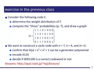
1. exercise in the previous class • Consider the following code C. • determine the weight distribution of C • compute the “three” probabilities (p. 7), and draw a graph • We want to construct a cyclic code with n = 7, k = 4, and m =3. • confirm that G(x) = x3 + x2 + 1 can be a generator polynomial • encode 0110 • decide if 0001100 is a correct codeword or not Answers: http://apal.naist.jp/~kaji/lecture/

2. today’s class • soft-decision decoding • make use of “more information” from the channel • convolutional code • good for soft-decision decoding • Shannon’s channel coding theorem • error correcting codes of the next generation

3. the channel and modulation • We considered “digital channels”. • At the physical-layer, almost all channels are continuous. digital channel=modulator + continuous channel + demodulator 0010 0010 0010 0010 modulator (変調器) continuous (analogue) demodulator (復調器) a naive demodulator translates the waveform to 0 or 1  the risk of possible errors

4. “more informative” demodulator From the viewpoint of error correction, the waveform contains more information than the binary output of the demodulator. • demodulators with multi-level output can help error correction. definitely 0 maybe 0 maybe 1 definitely 1 0 to make use of this multi-level demodulator, the decoding algorithm must be able to handle multi-level inputs 1

5. hard-decision vs. soft-decision • hard-decision decoding • the input to the decoder is binary (0 or 1) • decoding algorithms discussed so farare hard-decision type • soft-decision decoding • the input to the decoder can have three or more levels • the “check matrix and syndrome” approach does not work • more powerful, BUT, more complicated

6. formalization of the soft-decision decoding • outputs of the demodulator • 0+ (definitely 0), 0- (maybe 0), 1- (maybe 1), 1+ (definitely 1) • code C = {00000, 01011, 10101, 11110} • for a received vector 0- 0+ 1+ 0- 1-, find a codeword which minimizes the penalty . r 0- 0+ 1+ 0- 1- received 0+ 0- 1- 1+ penalty of “0” 0 1 2 3 penalty of “1” 3 2 1 0 = 0 0 0 0 0 c0 + + + + = 1 0 3 1 2 7 c2 = 1 0 1 0 1 + + + + = 2 0 0 1 1 4 (hard-decision ... penalty = Hamming distance)

7. algorithms for the soft-decision decoding We just formalized the problem... how can we solve it? • by exhaustive search? • ... not practical for codes with many codewords • by matrix operation? • ... yet another formalization which is difficult to solve • by approximation? • ... yes, this is one practical approach anyway... • design special codes; • whose soft-decision decoding is not “too difficult”  convolutional code (畳み込み符号)

8. convolutional codes • the codes we studied so far... block codes • a block of k-bit data is encoded to a codeword of length n • the encoding is done independently for block to block • convolutional codes • encoding is done in a bit-by-bit manner • previous inputs are stored in shift-registers in the encoder, and affects future encoding input data combinatorial logic encoder outputs

9. r3 r2 r1 encoding of a convolutional code • at the beginning, the contents of registers are all 0 • when a data bit is given, the encoder outputs several bits, and the contents of registers are shifted by one-bit • after encoding, give 0’s until all registers hold 0 encoder example constraint length = 3 ( = # of registers) the output is constrained by three previous input bits

10. 1 0 1 1 1 0 1 1 0 1 0 1 1 0 0 0 0 0 1 1 0 1 1 0 encoding example (1) • to encode 1101... give additional 0’s to push-out 1’s in the register...

11. 1 0 0 0 0 1 0 0 0 0 1 0 1 0 1 1 0 1 0 1 1 0 0 0 encoding example (2) the output is 11 10 01 10 00 00 01

12. 00 s0 r2 r1 11 01 input 00 s1 s2 output 10 11 01 s3 0 1 10 encoder as a finite-state machine constraint length k  the encoder has 2k internal states internal state = (r2, r1) s0=(0, 0), s1=(0, 1), s2=(1, 0), s3=(1, 1) • the encoder is a finite-state machine • whose initial state is s0 • makes one transition for each input bit • returns to s0 after all data bits are provided

13. 01001... 01100... errors encoder receiver at the receiver’s end • the receiver knows... • the definition of the encoder (finite-state machine) • the encoder starts and ends at the state s0 • the transmitted sequence which can be corrupted by errors to correct errors = to estimate the “real” transition of the encoder ... estimation on a hidden Markov model (HMM)

14. s0 s2 s1 trellis diagram a trellis diagram is obtained by... expanding the transition of the encoder to the time axis trellis s0,0 s5,0 s0 s1 expansion s2 time 0 1 2 3 4 5 • possible encoding sequences (of length 5) = the set of paths connecting s0,0 and s5,0 • the transmitted sequence = the path which is the most-likely to the received sequence = the path with the minimum penalty

15. Viterbi algorithm given a received sequence... • the demodulator defines penalties for symbols at each position • the penalties are assigned to edges of the trellis diagram • find the path with the minimum penalty using a good algorithm Viterbi algorithm • the Dijkstra algorithm for HMM • recursive width-first search pA qA the minimum penalty of this state is min (pA+qA, pB+qB) s0,0 Andrew Viterbi 1935- qB pB

16. soft-decision decoding for convolutional codes the complexity of Viterbi algorithm ≈ the size of the trellis diagram • for convolutional codes (with constraint length k): • the size of trellis ≈ 2k×data length ... manageable • we can extract 100% performance of the code • for block codes: • the size of trellis ≈ 2data length ... too large • it is difficult to extract the full performance moderated performance, full power available convolutional code good performance, but difficult to use block code performance

17. summary of the convolutional codes advantage: • the encoder is realized by a shift-register (like as cyclic codes) • soft-decision decoding is practically realizable disadvantage: • no good algorithm for constructing good codes • code design = the wire connection of register outputs • design in the “trial-and-error” manner with computer

18. channel capacity mutual information I(X; Y): • X and Y: the input and output of the channel • the average information of X given by Y • depends on the statistical behavior of the input X • channel capacity = max I(X; Y) ... the maximum performance achievable by the channel X Y

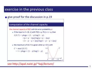
19. computation of the channel capacity the channel capacity of BSC with bit error probability p: • if the input is X = {0, 1} with P(0) = q, P(1) = 1 – q, then • the maximum of I(X; Y) is given when q = 0.5, with C 1.0 0.5 p 0 0.5 1.0

20. Shannon’s channel coding theorem • code rate R = log2(# of codewords) / (code length) (= k / n for an (n, k) binary linear code) Shannon’s channel coding theorem: consider a communication channel with capacity C; • a code with rate R ≤ C, with which error at the receiver → 0 • no such code exists if the code rate R > C The theorem says that such a code exists at “some place”. ... How can we reach there?

21. investigation towards the Shannon’s limit by mid 1990s ... “combine several codes” approach • concatenated code (連接符号) • apply multiple error correcting codes sequentially • typically; Reed-Solomon + convolutional codes encoder 1 encoder 2 outer code (RS code) inner code (conv. code) channel decoder 1 decoder 2

22. 0 1 0 1 0 0 1 0 1 1 0 1 0 0 1 1 1 0 0 1 1 0 1 1 0 1 0 0 1 0 1 0 1 1 0 0 1 0 0 1 0 0 0 1 1 0 1 0 1 product code • product code (積符号) • 2D code with more powerful codes applied for row/column data bits parities of code 1 decoding of code 2 decoding of code 1 possible problem: in the decoding of code 1, the received information is not considered parities of code 2

23. 0 1 0 1 0 0 1 0 1 1 0 1 0 0 1 1 1 0 0 1 1 0 1 1 0 1 0 0 1 0 1 0 1 1 0 0 1 0 0 1 0 0 0 1 1 0 1 0 1 idea for the breakthrough • let the decoder see two inputs: • the result of the previous stage + received information • feed-back the decoding result of code 1, and try decode code 2 Exchange the decoding results between two decoders iteratively. 二台の復号器間で，復号結果を繰り返し交換する data bits parities of code 1 decoding of code 2 decoding of code 1 parities of code 2

24. the iterative decoding idea: product code + iterative decoding decoder for code 1 received sequence decoder for code 2 decoding result • the decoder is modified to have two inputs • two soft-value inputs and one soft-value output • trellis-based maximum a-posteriori decoding • the result of one decoder helps the other decoder  more # of iteration, more reliable result

25. data bits parity: code 1 parity: code 2 coded sequence Turbo code: encoding Turbo code: • Add two sets of parities for one set of data bits • Use convolutional codes for the simplicity of decoding data bits coded sequence encode: code 1 interleaver encode: code 2 (bit reorder)

26. received sequence decoding result decoder: code 1 I–1 I decoder: code 2 I interleaver I I–1 de-interleaver Turbo code: decoding • Each decoder sends its estimation to the other decoder. • Experiments shows that... • code length must be sufficiently long (> thousands bits) • the # of iterations can be small (≈ 10 to 20 iterations)

27. performance of Turbo codes • The performance is much better than other known codes. • There is some “saturation (飽和)” of the performance improvement. (error-floor) C. Berrou et al.: Near Shannon Limit Error-Correcting Coding and Decoding: Turbo Codes, ICC 93, pp. 1064-1070, 1993.

28. LDPC code The study of Turbo codes revealed that “the length is the power”. • don’t bother too much on mathematical properties • pursue long and easily decodable codes LDPC code(Low Density Parity Check code) • linear block code with very sparse check matrix • almost all components are 0, with small # of 1 • discovered by Gallager in 1962, but forgotten for long years • MacKay’s rediscovery in 1999 David MacKay 1967- Robert Gallager 1931-

29. 1 1 1 0 1 0 0 1 0 1 1 0 1 0 0 1 1 1 0 0 1 H = p1 p3 p4 p6 prob. of 0 q1 q3 q4 q6 prob. of 1 (= 1 – pi) the decoding of LDPC codes • An LDPC code is a usual linear block code, but its sparse check matrix allows belief-propagation algorithm to work efficiently and effectively. Tanner Graph p3 = p1 p4 p6 + q1 q4 p6 + q1 p4 q6 + p1 q4 q6

30. LDPC vs. Turbo codes • performance: • both codes show excellent performance • the decoding complexities are “almost linear” • LDPC shows “more mild” error-floor phenomenon • realization: • O(n) encoder for Turbo, O(n2) encoder for LDPC • code design: • LDPC has more varieties and strategies

31. summary • soft-decision decoding • retrieve more information from the channel • convolutional code • good for soft-decision decoding • Shannon’s channel coding theorem • what we can and we cannot • error correcting codes of the next generation

32. exercise • give proof for the discussion in p.19