Download
1 / 72
720 likes | 778 Views
Learn how to use Safety Performance Functions (SPFs) and Crash Modification Factors (CMFs) to predict crash frequency on rural highways. Explore the influence of cross-sectional elements on safety and operations.

E N D
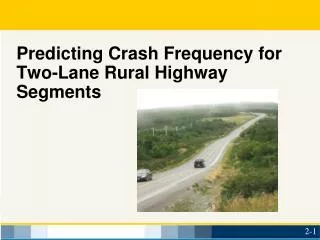
Predicting Crash Frequency for Two-Lane Rural Highway Segments
Predicting Crash Frequency for Two-Lane Rural Highway Segments • Describe the Safety Performance Functions (SPFs) for predicting Crash Frequency for Base Conditions • Describe the Quantitative Safety Effects of Crash Modification Factors (CMFs) • Apply CMFs to the SPF Base Equation Learning Outcomes:
Predicting Crash Frequency for Two-Lane Rural Highway Segments Cross Sectional Elements
Lane Width Shoulder Width Sideslope Clear Zone Crashes Operations Head-on Capacity Wider is “better” Wider means “faster” Run-off-Road Capacity Wider is “better” Functionality (peds, bikes, emergency stops, capacity, maintenance) Run-off-road Maintenance (severity) Flatter is better Flatter is better Run-off-road Horizontal sight distance (frequency and severity) Two-Lane Rural Highway Segments What should you expect would be the safety and operational influence of cross sectional elements?
Protection for turns off the roadway Provide pavement support Store snow Provide space for maintenance activities Enforcement activities Clear zone (recovery) Highway Capacity Clear zone (horizontal sight distance) Store vehicles in emergency Pedestrians, bicyclists Two-Lane Rural Highway Segments Functions of shoulders in a rural environment
Two-Lane Rural Highway Segments Key Findings of FHWA Cross Section Study on Two-Lane Hwys (Zegeer) • Traffic volume influences crash rate • Both lane and shoulder width have influence • Roadside Hazard next biggest influence on crashes • Alignment affects cross section crashes (terrain is surrogate for alignment)
Two-Lane Rural Highway Segments Crash Severity for Two-Lane Rural Highways Rural 2 Lane Highway Segment Severity Ratio = 32.1% for Injury + Fatal Crashes
HSM Crash Prediction: 18 Steps for Two-Lane Rural Roadways Rural Area Definition: • Places outside urban boundaries • Populations of 5,000 persons, or less Applicable to: • Existing Roadways • Design Alternatives for existing or new roadways
Predicting Crash Frequency Performance - Analysis Sections Organizing information for Safety Analysis: • Separate project lengths (and crashes) into homogeneous units: • Average daily traffic (AADT) volume (vehicles/day) • Lane width (ft) • Shoulder width (ft) • Shoulder Type • Driveway Density (driveways per mile) • Roadside Hazard Rating • Beginning/End of Horizontal Curves • Beginning/End of Segments on Grade (>3%)
Subdividing Roadway Segments Lane Width • Homogeneous Roadway Segments:
Subdividing Roadway Segments Shoulder Width • Homogeneous Roadway Segments:
HSM Crash Prediction Method Three Basic Elements: 1.Safety Performance Functions (SPF) Equations • Predict safety performance for set base conditions 2.Crash Modification Factors (CMFs) • Adjust predicted safety performance from base conditions to existing/proposed conditions • Are greater or less than 1: • < 1.0 -- lower crash frequency • > 1.0 -- increased crash frequency • Calibration, Cr or Ci • Accounts for local conditions/data
Total estimated crashes within the limits of the roadway being analyzed: HSM Crash Prediction Method Ntotal = ∑Npredicted-rs + ∑ Npredicted-int Ntotal = Total expected number of crashes within the limits of the roadway facility ∑Npredicted-rs = Expected crash frequency for all roadway segments (sum of individual segments) ∑ Npredicted-int = Expected crash frequency for all intersections (sum of individual intersections)
Roadway Segment Prediction Model Npredicted-rs = Nspf-rs x (CMF1r … CMFxr) Cr Where: • Npredicted-rs = predicted average crash frequency for an individual roadway for a specific year (crashes per year) • Nspf-rs = predicted average crash frequency for base conditions for an individual roadway segment (crashes per year) • CMF1r ... CMFxr = Crash Modification Factors for individual design elements • Cr = calibration factor
SPF for Two-Lane Rural Highway Segment Crashes for Base Conditions: Safety Performance Function (SPF) Where: • Nspf-rs = predicted total crash frequency for a roadway segment for base conditions, crashes per year • AADTn = average annual daily two-way traffic volume for specified year n (veh/day) • L = length of roadway segment (miles) Nspf-rs = (AADTn) (L) (365) (10-6) e-0.312
Base Conditions for Rural Two-Lane Roadway Segments (CMF = 1.0) • Lane Width: 12 feet • Shoulder Width: 6 feet • Shoulder Type: Paved • Roadside Hazard Rating: 3 • Driveway Density: <5 driveways/mi • Grade: <3%(absolute value) • Horizontal Curvature: None • Vertical Curvature: None • Centerline rumble strips: None • TWLTL, climbing, or passing lanes: None • Lighting: None • Automated Enforcement: None
Safety Performance Function (SPF) Applying SPF for Base Conditions – Example: 2-lane state highway connecting a US marked route to a primary State marked route in a rural county; Where: AADT = 3,500 vpd Length = 26,485 feet = 5.02 miles Nspf-rs = (AADTn) (L) (365) (10-6) e-0.312
Safety Performance Function (SPF) Applying SPF for Base Conditions – Example: Where: AADT = 3,500 vpd Length = 26,485 feet = 5.02 miles Nspf-rs = (AADTn) (L) (365) (10-6) e-0.312 Nspf-rs = (3,500) (5.02) (365) (10-6) e-0.312 = (3,500) (5.02) (365) (10-6) (0.7320) = 4.69 crashes per year
Next Step is: Applying CMF’s for Conditions other than “Base” Npredicted-rs = Nspf-rs x (CMF1r … CMFxr) Cr Where: • Npredicted-rs = predicted average crash frequency for an individual roadway for a specific year (crashes per year) • Nspf-rs = predicted average crash frequency for base conditions for an individual roadway segment (crashes per year) • CMF1r ... CMFxr = Crash Modification Factors for individual design elements • Cr = calibration factor
Crash Modification Factors (CMFs) • CMFs quantify the expected change in crashes at a site caused by implementing a particular treatment, countermeasure, intervention, action, or alternative. • CMFs are used to adjust the SPF estimated predicted average crash frequency for the effect of individual geometric design and traffic control features.
Crash Modification Factors (CMFs) Applying CMFs for Lane Width, Shoulder Width & Type, Driveway Density, TWTLs, and Roadside Design Npredicted-rs = Nspf-rs(CMF1r x CMF2r x CMF6r x CMF9r x CMF10r) Where: CMF1r is for Lane Width CMF2r is for Shoulder Width and Type CMF6r is for Driveway Density CMF9r is for Two-Way Left-Turn Lanes CMF10r is for Roadside Design Nspf-rs = (AADTn) (L) (365) (10-6) e-0.312
Crash Modification Factor for Lane Width (CMF1r) CMF1r = (CMFra – 1.0)pra + 1.0 • ‘Base condition’ is 12-ft lanes • CMFs for ADT >2000 based on Zegeer • CMFs for ADT <400 based on studies by Griffin and Mak • Expert panel developed transition lines, referencing other research CMFra for lane width 1.23
Crash Modification Factor for Lane Width (CMF1r) CMF1r = (CMFra – 1.0)pra + 1.0 Note equations for ADT’s between 400 and 2000
CMF - Lane and Shoulder Width Adjustment for Related Crashes Table 10-4 - Adjust for (Run off Road + Head-on + Sideswipes) to total crashes pra = 0.574 CMF1r = (CMFra – 1.0)pra + 1.0
Calculation for Lane Width (CMF1r): Example For 3,500 AADT for a 10 foot wide lane: From Table 10-8: CMFra = 1.30 • Adjustment for lane width and shoulder width related crashes (Run off Road + Head-on + Sideswipes) to obtain total crashes using default value for pra = 0.574 CMF1r = (CMFra - 1.0) pra + 1.0 = (1.30 - 1.0) * 0.574 + 1.0 = (0.30) (0.574) + 1.0 = 1.172
Calculation for Shoulder Width and Type (CMF2r) CMF2r = (CMFwraCMFtra– 1.0)pra + 1.0 CMFwra for shoulder width: • Base condition is 6-ft shoulders • CMFs for ADT >2000 based on Zegeer (FHWA) • CMFs for ADT <400 based on other studies by Zegeer (NCHRP 362) • Expert panel developed transition lines, referencing other research
Crash Modification Factor for Shoulder Width (CMFwra) CMF2r = (CMFwraCMFtra– 1.0)pra + 1.0 Note equations for ADT’s between 400 and 2000
CMF – Lane and Shoulder Width Adjustment for Related Crashes Table 10-4 - Adjust for (Run off Road + Head-on + Sideswipes) to total crashes pra = 0.574 CMF2r = (CMFwraCMFtra – 1.0)pra + 1.0
Calculation for Shoulder Width and Type (CMF2r): Example For 3,500 AADT with a 2 ft wide aggregate shoulder: CMFwra = 1.30 (Table 10-9) and CMFtra = 1.01 (Table 10-10) • Adjustment from crashes related to lane and shoulder width (Run off Road + Head-on + Sideswipes) to total crashes using default value for pra = 0.574 CMF2r = (CMFwra CMFtra - 1.0) pra + 1.0 = ((1.30)(1.01) - 1.0) * 0.574 + 1.0 = (0.313) (0.574) + 1.0 = 1.180
Crash Modification Factors Lane and Shoulder Width – Example: • For 1,500 AADT 10’ lane and no shoulder: What is CMF1r&2r? • Lane Width = 10’ • (From Table 10-8)CMFra = 1.213 • CMF1r = (1.213 - 1.0)x 0.574 + 1.0 = 1.122 • Shoulder Width = 0’ (From Table 10-9) CMFwra = 1.375 CMF2r= (((1.375 x 1.00) -1.0)x 0.574) + 1.0 = 1.215 Combined CMF: CMF1r&2r = 1.122x 1.215 = 1.363
Crash Modification FactorsExample: Combination Shoulder Type 6 ft Shoulder, AADT > 2,000 vpd From Table 10-10: • CMF6’ paved = 1.00 • CMF6’ gravel = 1.02 6 ft 4’ 2’ • Combination Shoulder Type CMFtra Calculation: • CMFtra =(4’/6’)x1.00 + (2’/6’) x 1.02 = 1.007
Some Insights Review of CMFs for Lane Width and Shoulders • Not much difference between 11- and 12-ft lanes • Lane width is less important for very low volume roads • Incremental width for shoulders is much more sensitive than for lanes • Shoulder width effectiveness increases significantly as AADT increases
CMF for % Grade for Roadway Segments (CMF5r) For Roadway Segment on 4% Grade: CMF5r = ? 1.10
CMF for Driveway Density (Access) (CMF6r) Where: CMF6r = effect of driveway density on total crashes DD = Driveway Density (driveways per mile) AADT = Average Annual Daily Traffic 0.322 + (0.05-0.005Ln(AADT))*DD _____________________ CMF6r = 0.322 + (0.05-0.005*Ln(AADT))*5
Calculation for Driveway Density (CMF6r): Example Where: AADT = 3,500 Access is 31 driveways in 5.02 miles DD = 31/5.02 = 6.17 driveways per mile 0.322 + (0.05-0.005*Ln(AADT))*DD _____________________ CMF6r = 0.322 + (0.05-0.005*Ln(AADT))*5 0.322 + (0.05-0.005*Ln(3,500))*6.17 = 0.322 + (0.05-0.005*Ln(3,500))*5 = 1.029
Safety Effects of Installing Shoulder Rumble Strips: Two-Lane Rural Roads * Not in HSM *CRFrumble = 13% reduction in total crashes CMF = 1 – *CRF CMFrumble = 1- 0.13 = 0.87 *From FHWA CMF Clearinghouse http://www.cmfclearinghouse.org
CMF for Rural Two-Way Left Turn Lanes (CMF9r) • Most effective where one direction flow rate > 300 vph and in rural areas
CMF for TWLTL Lanes (CMF9r) CMF9r = 1.0 – 0.7 PD * PLT/D Where: Pdwy = Driveway-related crashes as a proportion of total crashes Pdwy = (0.0047 DD + 0.0024 DD2) (1.199 + 0.0047 DD + 0.0024 DD2) DD= drive density (driveways/mi > 5/mile) PLT/D = Left turn crashes susceptible to correction by a TWLTL as a proportion of driveway related crashes (estimated as 0.50)
Example Calculation for TWLTL (CMF9r) CMF9r = 1.0 – (0.7 Pdwy x PLT/D) For 35 driveways in 0.8 mile long segment DD = 35/0.8 = 43.47 driveways/mi Pdwy = (0.0047(43.47)) + 0.0024(43.472) (1.199 + 0.0047(43.47) + 0.0024(43.472) = 0.80 CMF9r = 1.0 – (0.7 x 0.80 x 0.50) = 0.72
Roadside Quality is Strongly Linked to Related CrashesRoadside Design (CMF10r) • Roadside Design is based on Roadside Hazard Ratings that are dependent on the roadside environment • Ratings range from 1 to 7: • 1 = forgiving roadside environment • 7 = unforgiving roadside environment
Roadside Hazard Ratings Base condition is Hazard Rating = 3
Roadside Hazard Rating of 1 • Wide clear zones greater than or equal to 30 ft from the pavement edgeline. • Sideslopes flatter than 1:4 • Recoverable sideslope
Roadside Hazard Rating of 2 4 1 • Clear zone between 20 and 25 ft from pavement edgeline • Sideslope about 1:4 • Recoverable sideslope
Roadside Hazard Rating of 3 3 1 • Clear zone about 10 ft from pavement edgeline • Sideslope about 1:3 or 1:4 • Rough roadside surface • Marginally recoverable
Roadside Hazard Rating of 4 • Clear zone between 5 and 10 ft from pavement edgeline • Sideslopes about 1:3 or 1:4 • May have guardrail (5 to 6.5 ft from pavement edgeline). • May have exposed trees, poles, or other objects (about 10 ft from pavement edgeline) • Marginally forgiving, but increased chance of a reportable roadside crash
Roadside Hazard Rating of 5 • Clear zone between 5 and 10 ft from pavement edgeline • Sideslope about 1:3 • Virtually non-recoverable • May have guardrail (0 to 5 ft from edgeline) • May have exposed trees, poles, or other objects (about 10 ft from pavement edgeline)