Download
1 / 39
390 likes | 406 Views
This report explores the accurate implementation of the source wavelet in seismic modeling procedures and highlights the importance of information beyond travel time. It discusses the issues of the source term and proposes a method for implementing the source using a distribution of grids.

E N D
Accurate implementation of the source wavelet in finite-difference modeling Fang Liu and Arthur Weglein Annual report: page 111-125 Houston, Texas May 12th, 2006
Why ? Many seismic modeling procedures emphasis the travel time of the events, rather than the full wave-form. Information beyond correct travel-time, especially accurate implement of the source wavelet. Inverse scattering series preferred actual wave-fields.
Outline • Introduction • Source implementation • A very simple quality procedure • Physical meaning of discrete model • Issues of free surface • Conclusion
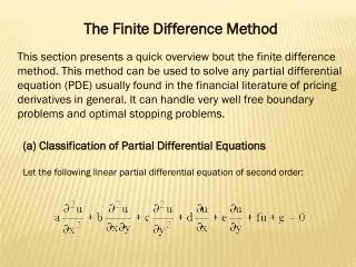
Introduction Forward modeling problem: differential equation Velocity model Source wavelet Very well-known unsolvable problem with analytic solution
Finite difference approximation partial derivative over time Previous time Current time Future time (Second order in time)
Finite difference approximation spatial partial derivatives (Fourth order in space)
Finite difference approximation of LHS of wave-equation How about the RHS ?
Source implementation Issues of the source: A source invisible to the grids Grid points
Issues of the source term A source visible to the grids Grid points But the wave-field at the source point will be singular
Convert the source problem to an initial problem Source problem Initial problem without source The above 2 problem will produce the same response because the first one will evolve into the second. After certain time, the source become very weak and hence negligible. But the second problem is much easier because it contains no source. And the source is implemented by a distribution of grids rather than in the single source point, source can be flexibly put between grids.
How the source is implemented wave-fields at previous time wave-fields at future time current wave-fields
Advantages • The new problem is much simpler to solve. • Source can be flexibly put on the grids or in between. • Singular source is implemented by a regular distribution of points.
Procedures to propagate forward in time Previous step Next step (future time) Current step (current time)
Modeling parameters We want the digitization interval the smaller the better. But computer set the lower-limit for them. Lower limit of the digitization interval constrains the frequency content of the source wavelet.
A simple quality control procedure For the modeling parameters • Construct a model with the same set of velocity contrast but no lateral variation • Run forward modeling with point source • Summing all receivers together • Compare with analytic solution 1500(m/s) 1500(m/s) 2000(m/s) 2000(m/s) 1500(m/s) 1500(m/s)
Summing over receivers Define: Summing all receivers We have an equivalent 1D wave-equation:
Source issue for a 3rd party program Geological model The receiver line (depth=25m) Source depth=0m The first reflector (depth = 497.5m) The second reflector (depth = 897.5m)
It was given maximal freedom to decide parameters Model designed very big to minimize boundary artifacts We only specify : Give the standard package the maximal freedom to decide Velocity contrast set to be small to minimize other issues
What’s the problem ? Waveform of each event: 1500(m/s) 2000(m/s) Positive and negative half should be symmetrical 1500(m/s) Size of first Peak Size of second Peak Events Difference Direct wave -29.995 30.274 0.93 % First primary -3.719 4.941 32.86 % Second primary 35.59 % 3.574 -4.846
Our results for the same parameters First primary -7420 7414 0.08 % Second primary 0.05 % 7414 -4.846
Example 1 : geological model and modeling parameters Source and receivers line (depth=0m) 997.5m 1497.5m
Example 1 : Summing of all receivers Sum from finite-difference data Analytic integral from equation (14)
First experiment with Ricker wavelet (without free-surface) (1) Pre-calculated wave field 0 m 1500 (m/s) 997.5 m R1 = 0.23077 3200 (m/s) 1497.5 m R2’ = 0.2952 6100 (m/s) Field pre
My own experiment with Ricker wavelet Recovering zero frequency by integrating twice Problem only for large time
Physical meaning of discrete model Velocity model within computer memory Where is the reflector? Interpretation above is very important for free-surface implementation.
Analytic using z1=997.5 (m) Sum from finite-difference data Analytic using z1=995 (m) Analytic using z1=1000 (m)
Experiment with Ricker wavelet with free-surface Location of free-surface is critical because it determine the location of the image source, and affect the pre-calculated wave-field 0: 1: Δx=Δz=5 free-surface (2.5 m) 2: 3: 79: water bottom (397.5 m) Water-bottom reflection coef:
Ricker wavelet with dominant freq=17 HZ Correct free-surface (level=2.5m)
Ricker wavelet with dominant freq=17 HZ Summing all traces together Still a little high-frequency noise But better than 17 hz
Ricker wavelet with dominant freq=17 HZ Amplitude check 5.57(cm) Primary+ghost 2nd multiple+ghost 0.7 (cm) 1st multiple+ghost -2 (cm)
In the plane-wave world, amplitude of each events have very simple relations Image source Free-surface Source Water-bottom Amplitude (Primary) =-R Amplitude (1st free-surface multiple) Amplitude (1st free-surface multiple) =-R Amplitude (2nd free-surface multiple)
Ricker wavelet with dominant freq=17 HZ Wrong free-surface (level=0m) Shot gather looks very similar as before
Ricker wavelet with dominant freq=17 HZ Summing all traces together But the result as summing all traces together is totally unreasonable
Ricker wavelet with dominant freq=17 HZ Summing all traces together High-frequency noise a little weaker
Conclusions • Accurate implementation of the source wavelet. • Simple quality-control for modeling parameters. • Physical meaning of the digitized model. • Implementation of the free-surface.
Acknowledgements M-OSRP members M-OSRP sponsors NSF-CMG award DMS-0327778 DOE Basic Sciences award DE-FG02-05ER15697