Download
1 / 25
260 likes | 456 Views
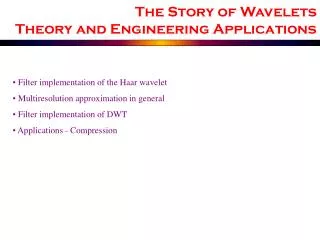
The Story of Wavelets Theory and Engineering Applications. Filter implementation of the Haar wavelet Multiresolution approximation in general Filter implementation of DWT Applications - Compression. a(j-1, 2k+1). a(j,k). f j (t). f(t). f j-1 (t). a j,k. a j,2k. a j-1,k. h’[n]. 2.

E N D
The Story of WaveletsTheory and Engineering Applications • Filter implementation of the Haar wavelet • Multiresolution approximation in general • Filter implementation of DWT • Applications - Compression
a(j-1, 2k+1) a(j,k) fj(t) f(t) fj-1(t) aj,k aj,2k aj-1,k h’[n] 2 a(j-1,2k) DWT Using Filtering Note that at the next finer level, intervals are half as long, so you need 2k to get the same interval. h’[n] yj-1,k aj-1,k Approx. coefficients at any level j can be obtained by filtering coef. at level j-1 (next finer level) by h’[n] and downsampling by 2
dj,k dj,2k aj-1,k g’[n] 2 Filter Implementation of Haar Wavelet We showed that aj,k can be obtained from aj-1,k through filtering by using a filter followed by a downsampling operation (drop every other sample). Similarly, dj,k can also be obtained from aj-1,kusing the filter g’[n] followed by down sampling by 2… Detail coefficients at any level j can be obtained by filtering approximation coefficients at level j-1 (next finer level) by g’[n] and downsampling by 2 This is called decomposition in the wavelet jargon.
Decomposition Filters • If we take the FT of h’[n] and g’[n]… LPF HPF
Decomposition / Reconstruction Filters • We can obtain the coarser level coefficients aj,k or dj,k by filtering aj-1,k with h’[n] or g’[n], respectively, followed by downsampling by 2. • Would any LPF and HPF work? No! There are certain requirements that the filters need to satisfy. In fact, the filters are obtained from scaling and wavelet functions using dilation (two-scale) equations (coming soon…) • Can we go the other way? Can we obtain aj-1,k from aj,k and dj,k from a set of filters. YES!. This process is called reconstruction. • Upsample a(k,n) and d(k,n) by 2 (insert zeros between every sample) and use filters h[n]=[n]+ [n-1] and g[n]= [n]- [n-1]. Add the filter outputs !
g`[n] 2 2 2 2 2 2 2 2 h`[n] g[n] g[n] g`[n] + + h[n] h[n] h`[n] The Discrete Wavelet Transform aj,k aj,k dj+1,k aj+1,k aj+1,k dj+2,k aj+2,k Decomposition Reconstruction We have only shown the above implementation for the Haar Wavelet, however, as we will see later, this implementation – subband coding – is applicable in general.
• We see that app. and detail coefficients can be obtained through filtering operations, but where do scaling and wavelet functions appear in the subband coding DWT implementation? • Clearly, these functions are somehow hidden in the filter coefficients, but how? • To find out, we need to know little bit more about these scaling and wavelet functions
2 1 MRA on Discrete Functions • Let’s suppose that the function f(t) is sampled at N points to give the sequence f[n], and further suppose that kthresolution is the highest resolution (we will compute approximations at k+1, k+2, …etc. Then: • Multiplying and integrating 1 2 h[k] g[k]
2 2 From MRA to Filters • This substitution gives us level j+1 approximation and detail coefficients in terms of level j coefficients : we can put the above expressions in convolution (filter) form as ~ H aj+1,k aj,k 1-level of DWT decomposition ~ G dj+1,k ~ ~ h[n]=h[-n], and g[n]=g[-n] So where do these filters really come from…?
Dilation / Two-scale Equations • Two scale (dilation) equations for the scaling and wavelet functions determine the filters associated with these functions. In particular: • The coefficients c(n) can be obtained as • Recall that • In some books, h[k]= c(k)/√2. Then the two-scale equation becomes or more generally
Dilation / Two-scale Equations • Similarly, the two-scale equation for the wavelet function: • Then: ~ In some books, g[k]= b(k)/√2. Then the two-scale equation becomes
Two-Scale Equations • These two equations determine the coefficients of all 4 filters: h[n]: Reconstruction, lowpass filter g[n]: Reconstruction, highpass filter h[n]: Decomposition, lowpass filter g[n]: Decomposition, highpass filter • The following observations can therefore be made ~ ~ ~ Note : |H(jw)|= |H(jw)|
Quadrature Mirror Filters • It can be shown that that is, h[] and g[] filters are related to each other: in fact, that is, h[] and g[] are mirrors of each other, with every other coefficient negated. Such filters are called quadrature mirror filters. For example, Daubechies wavelets with 4 vanishing moments…..
DB-4 Wavelets ~ h = -0.0106 0.0329 0.0308 -0.1870 -0.0280 0.6309 0.7148 0.2304 g = -0.2304 0.7148 -0.6309 -0.0280 0.1870 0.0308 -0.0329 -0.0106 h = 0.2304 0.7148 0.6309 -0.0280 -0.1870 0.0308 0.0329 -0.0106 g = -0.0106 -0.0329 0.0308 0.1870 -0.0280 -0.6309 0.7148 -0.2304 ~ L: filter length (8, in this case) Matlab command “wfilters()” Use freqz() to see its freq. response
G 2 2 2 2 2 2 2 2 H G G G + + H H H DWT implementation:Subband Coding x[n] x[n] ~ ~ ~ ~ Decomposition Reconstruction
|H(jw)| w /2 -/2 2 2 2 2 2 DWT Decomposition x[n] Length: 512 B: 0 ~ g[n] h[n] Length: 256 B: 0 ~ /2 Hz Length: 256 B: /2 ~ Hz |G(jw)| d1: Level 1 DWT Coeff. g[n] h[n] Length: 128 B: 0 ~ /4 Hz w Length: 128 B: /4 ~ /2 Hz -/2 /2 - d2: Level 2 DWT Coeff. g[n] h[n] 2 Length: 64 B: 0 ~ /8 Hz Length: 64 B: /8 ~ /4 Hz ……. d3: Level 3 DWT Coeff.
Applications Detect discontinuities
Applications Detect hidden discontinuities
Applications Simple denoising
Compression • DWT is commonly used for compression, since most DWT are very small, can be zeroed-out!