CHAPTER 8 Estimating with Confidence

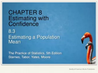
1. CHAPTER 8Estimating with Confidence 8.3 Estimating a Population Mean

2. When σ Is Unknown: The t Distributions When we don’t know σ, we can estimate it using the sample standard deviation sx. What happens when we standardize?

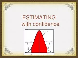
3. When σ Is Unknown: The t Distributions • When we standardize based on the sample standard deviation sx, our statistic has a new distribution called a t distribution. • It has a different shape than the standard Normal curve: • It is symmetric with a single peak at 0, • However, it has much more area in the tails. There is a different t distribution for each sample size, specified by its degrees of freedom (df).

4. The t Distributions; Degrees of Freedom When we perform inference about a population mean µ using a t distribution, the appropriate degrees of freedom are found by subtracting 1 from the sample size n, making df = n - 1. We will write the t distribution with n - 1 degrees of freedom as tn-1. Conditions for Constructing a Confidence Interval About a Proportion Draw an SRS of size n from a large population that has a Normal distribution with mean µ and standard deviation σ. The statistic has the t distribution with degrees of freedom df = n – 1. When the population distribution isn’t Normal, this statistic will have approximately a tn– 1 distribution if the sample size is large enough.

5. The t Distributions; Degrees of Freedom When comparing the density curves of the standard Normal distribution and t distributions, several facts are apparent: • The density curves of the t distributions are similar in shape to the standard Normal curve. • The spread of the t distributions is a bit greater than that of the standard Normal distribution. • The t distributions have more probability in the tails and less in the center than does the standard Normal. • As the degrees of freedom increase, the t density curve approaches the standard Normal curve ever more closely.

6. Example: Using Table B to Find Critical t* Values Problem: What critical value t* from Table B should be used in constructing a confidence interval for the population mean in each of the following settings? (a) A 95% confidence interval based on an SRS of size n = 12. Solution: In Table B, we consult the row corresponding to df = 12 - 1 = 11. We move across that row to the entry that is directly above 95% confidence level on the bottom of the chart. The desired critical value is t* = 2.201.

7. Example: Using Table B to Find Critical t* Values Problem: What critical value t* from Table B should be used in constructing a confidence interval for the population mean in each of the following settings? (b) A 90% confidence interval from a random sample of 48 observations. Solution: With 48 observations, we want to find the t* critical value for df = 48 - 1 = 47 and 90% confidence. There is no df = 47 row in Table B, so we use the more conservative df = 40. The corresponding critical value is t* = 1.684.

8. Conditions for Estimating µ As with proportions, you should check some important conditions before constructing a confidence interval for a population mean. Conditions For Constructing A Confidence Interval About A Mean • Random: The data come from a well-designed random sample or randomized experiment. • 10%: When sampling without replacement, check • that • • Normal/Large Sample: The population has a Normal distribution or the sample size is large (n ≥ 30). If the population distribution has unknown shape and n < 30, use a graph of the sample data to assess the Normality of the population. Do not use t procedures if the graph shows strong skewness or outliers.

9. Constructing a Confidence Interval for µ To construct a confidence interval for µ, • Use critical values from the t distribution with n - 1 degrees of freedom in place of the z critical values. That is,

10. One-Sample t Interval for a Population Mean The one-sample t interval for a population mean is similar in both reasoning and computational detail to the one-sample z interval for a population proportion One-Sample t Interval for a Population Mean When the conditions are met, a C% confidence interval for the unknown mean µ is where t* is the critical value for the tn-1 distribution with C% of its area between −t* and t*.

11. Example: A one-sample t interval for µ Environmentalists, government officials, and vehicle manufacturers are all interested in studying the auto exhaust emissions produced by motor vehicles. The major pollutants in auto exhaust from gasoline engines are hydrocarbons, carbon monoxide, and nitrogen oxides (NOX). Researchers collected data on the NOX levels (in grams/mile) for a random sample of 40 light-duty engines of the same type. The mean NOX reading was 1.2675 and the standard deviation was 0.3332. Problem: (a) Construct and interpret a 95% confidence interval for the mean amount of NOX emitted by light-duty engines of this type.

12. Example: Constructing a confidence interval for µ State: We want to estimate the true mean amount µ of NOX emitted by all light-duty engines of this type at a 95% confidence level. Plan: If the conditions are met, we should use a one-sample t interval to estimate µ. • Random: The data come from a “random sample” of 40 engines from the population of all light-duty engines of this type. • 10%?: We are sampling without replacement, so we need to assume that there are at least 10(40) = 400 light-duty engines of this type. • Large Sample: We don’t know if the population distribution of NOX emissions is Normal. Because the sample size is large, n = 40 > 30, we should be safe using a t distribution.

13. Example: Constructing a confidence interval for µ _ Do: From the information given, x = 1.2675 g/mi and sx = 0.3332 g/mi. To find the critical value t*, we use the t distribution with df = 40 - 1 = 39. Unfortunately, there is no row corresponding to 39 degrees of freedom in Table B. We can’t pretend we have a larger sample size than we actually do, so we use the more conservative df = 30.

14. Example: Constructing a confidence interval for µ = (1.1599, 1.3751) Conclude: We are 95% confident that the interval from 1.1599 to 1.3751 grams/mile captures the true mean level of nitrogen oxides emitted by this type of light-duty engine.

15. Choosing the Sample Size We determine a sample size for a desired margin of error when estimating a mean in much the same way we did when estimating a proportion. Choosing Sample Size for a Desired Margin of Error When Estimating µ To determine the sample size n that will yield a level C confidence interval for a population mean with a specified margin of error ME: • Get a reasonable value for the population standard deviation σ from an earlier or pilot study. • Find the critical value z* from a standard Normal curve for confidence level C. • Set the expression for the margin of error to be less than or equal to ME and solve for n:

16. Example: Determining sample size from margin of error Researchers would like to estimate the mean cholesterol level µ of a particular variety of monkey that is often used in laboratory experiments. They would like their estimate to be within 1 milligram per deciliter (mg/dl) of the true value of µ at a 95% confidence level. A previous study involving this variety of monkey suggests that the standard deviation of cholesterol level is about 5 mg/dl. Problem: Obtaining monkeys is time-consuming and expensive, so the researchers want to know the minimum number of monkeys they will need to generate a satisfactory estimate.

17. Example: Determining sample size from margin of error Solution: For 95% confidence, z* = 1.96. We will use σ = 5 as our best guess for the standard deviation of the monkeys’ cholesterol level. Set the expression for the margin of error to be at most 1 and solve for n : Because 96 monkeys would give a slightly larger margin of error than desired, the researchers would need 97 monkeys to estimate the cholesterol levels to their satisfaction.