Introduction to Inference Estimating with Confidence

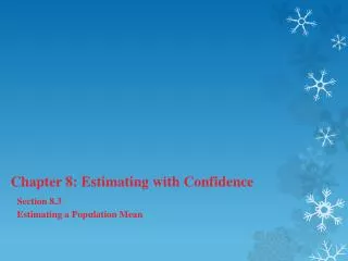
1. Introduction to InferenceEstimating with Confidence Chapter 6.1

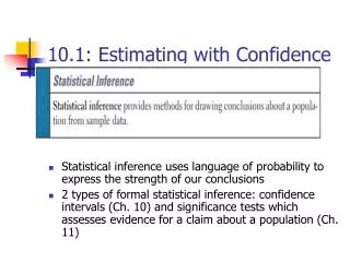
2. Overview of Inference • Methods for drawing conclusions about a population from sample data are called statistical inference • Methods • Confidence Intervals - estimating a value of a population parameter • Tests of significance - assess evidence for a claim about a population • Inference is appropriate when data are produced by either • a random sample or • a randomized experiment

3. x Statistical confidence Although the sample mean, , is a unique number for any particular sample, if you pick a different sample you will probably get a different sample mean. In fact, you could get many different values for the sample mean, and virtually none of them would actually equal the true population mean, .

4. n Sample means,n subjects But the sample distribution is narrower than the population distribution, by a factor of √n. Thus, the estimates gained from our samples are always relatively close to the population parameter µ. Population, xindividual subjects m If the population is normally distributed N(µ,σ), so will the sampling distribution N(µ,σ/√n),

5. 95% of all sample means will be within roughly 2 standard deviations (2*s/√n) of the population parameter m. Distances are symmetrical which implies that the population parameter m must be within roughly 2 standard deviations from the sample average , in 95% of all samples. Red dot: mean value of individual sample This reasoning is the essence of statistical inference.

6. The weight of single eggs of the brown variety is normally distributed N(65 g,5 g).Think of a carton of 12 brown eggs as an SRS of size 12. • What is the distribution of the sample means ? • Normal (mean m, standard deviation s/√n) = N(65 g,1.44 g). • Find the middle 95% of the sample means distribution. • Roughly ± 2 standard deviations from the mean, or 65g ± 2.88g. . • You buy a carton of 12 white eggs instead. The box weighs 770 g. The average egg weight from that SRS is thus = 64.2 g. • Knowing that the standard deviation of egg weight is 5 g, what can you infer about the mean µ of the white egg population? • There is a 95% chance that the population mean µ is roughly within ± 2s/√n of , or 64.2g ± 2.88 g.

7. Confidence intervals The confidence interval is a range of values with an associated probability or confidence level C. The probability quantifies the chance that the interval contains the true population parameter. ± 4.2 is a 95% confidence interval for the population parameterm. This equation says that in 95% of the cases, the actual value of m will be within 4.2 units of the value of .

8. n All we need is one SRS of size n and rely on the properties of the sample means distribution to infer the population mean m. n Sample Population m Implications We don’t need to take a lot of random samples to “rebuild” the sampling distribution and find m at its center.

9. Reworded With 95% confidence, we can say that µ should be within roughly 2 standard deviations (2*s/√n) from our sample mean . • In 95% of all possible samples of this size n, µ will indeed fall in our confidence interval. • In only 5% of samples would be farther from µ.

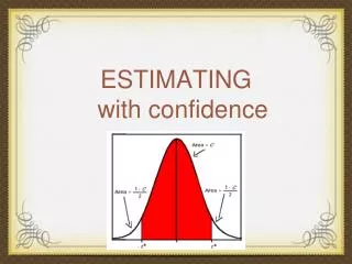
10. A confidence interval can be expressed as: • Mean ± mm is called the margin of errorm within ± mExample: 120 ± 6 • Two endpoints of an interval m within ( −m) to ( + m) ex. 114 to 126 A confidence level C (in %) indicates the probability that the µ falls within the interval. It represents the area under the normal curve within ± m of the center of the curve. m m

11. Review: standardizing the normal curve using z N(64.5, 2.5) N(µ, σ/√n) N(0,1) Standardized height (no units) Here, we work with the sampling distribution, and s/√n is its standard deviation (spread). Remember that s is the standard deviation of the original population.

12. Varying confidence levels Confidence intervals contain the population mean m in C% of samples. Different areas under the curve give different confidence levels C. • Practical use of z: z* • z* is related to the chosen confidence level C. • C is the area under the standard normal curve between −z* and z*. C −z* z* The confidence interval is thus: Example: For an 80% confidence level C, 80% of the normal curve’s area is contained in the interval.

13. How do we find specific z* values? We can use a table (Table D). For a particular confidence level, C, the appropriate z* value is just above it. Example: For a 98% confidence level, z*=2.326

14. C m m −z* z* Link between confidence level and margin of error The confidence level C determines the value of z* . The margin of error also depends on z*. Higher confidence C implies a larger margin of error m (thus less precision in our estimates). A lower confidence level C produces a smaller margin of error m (thus better precision in our estimates).

15. 96% confidence interval for the true density, z* = 2.054, and write = 28 ± 2.054(1/√3) = 28 ± 1.19 x 106 bacteria/ml 70% confidence interval for the true density, z* = 1.036, and write = 28 ± 1.036(1/√3) = 28 ± 0.60 x 106 bacteria/ml Different confidence intervals for the same set of measurements Density of bacteria in solution: Measurement equipment has standard deviation s = 1 * 106 bacteria/ml fluid. Three measurements: 24, 29, and 31 * 106 bacteria/ml fluid Mean: = 28 * 106 bacteria/ml.Find the 96% and 70% CI.

16. Impact of sample size The spread in the sampling distribution of the mean is a function of the number of individuals per sample. • The larger the sample size, the smaller the standard deviation (spread) of the sample mean distribution. • But the spread only decreases at a rate equal to √n. ⁄ √n Sample size n

17. Sample size and experimental design You may need a certain margin of error (e.g., drug trial, manufacturing specs). In many cases, the population variability (s) is fixed, but we can choose the number of measurements (n). So plan ahead what sample size to use to achieve that margin of error. Remember, though, that sample size is not always stretchable at will. There are typically costs and constraints associated with large samples. The best approach is to use the smallest sample size that can give you useful results.

18. What sample size for a given margin of error? Density of bacteria in solution: Measurement equipment has standard deviation σ = 1 * 106 bacteria/ml fluid. How many measurements should you make to obtain a margin of error of at most 0.5 * 106 bacteria/ml with a confidence level of 90%? For a 90% confidence interval, z* = 1.645. Using only 10 measurements will not be enough to ensure that m is no more than 0.5 * 106. Therefore, we need at least 11 measurements.