Upstream
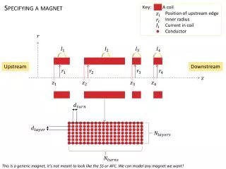
Specifying a magnet. Key: A coil Position of upstream edge Inner radius Current in coil Conductor. Upstream. Downstream. This is a generic magnet, it’s not meant to look like the SS or AFC. We can model any magnet we want!. Fitting a field map. Two methods:

Upstream
E N D
Presentation Transcript
Specifying a magnet Key: A coil Position of upstream edge Inner radius Current in coil Conductor Upstream Downstream This is a generic magnet, it’s not meant to look like the SS or AFC. We can model any magnet we want!
Fitting a field map • Two methods: • Mixing/scaling fit • Full 20+ parameter coil fit – takes FOREVER for SS • Mixing/Scaling fit procedure: • Take data in cylindrical co-ordinates • In this case using a pre-calculated map based on SS. • Make two detailed field maps with parameters that “bracket” our best guess at the real paramters • Minimise for “best fit” parameters: • Mixing of the detailed field maps • Length scale of the detailed field maps • Field scale of the detailed field maps
Fitting a field map • Mixing/Scaling fit procedure: • Take data in cylindrical co-ordinates • In this case using a pre-calculated map based on SS. Again, a generic magnet Spectrometer Solenoid parameters
Fitting a field map Mixing/Scaling fit procedure: Make two detailed field maps with parameters that “bracket” our best guess at the real parameters Original magnet “Long, thin” bracketing magnet “Short, fat” bracketing magnet
Fitting a field map • What do we mean by “detailed”? • Measured field on some grid • Bracket fields on finer grid, calculated over more points Mixing/Scaling fit procedure: Make two detailed field maps with parameters that “bracket” our best guess at the real parameters Long, thin bracketing magnet (): Example, all coils 3mm longer and thinner Short, fat bracketing magnet (): Example, all coils 3mm shorter and fatter
Fitting a field map • Mixing/Scaling fit procedure: • Minimise for “best fit” parameters: • Mixing of the detailed field maps • Length scale of the detailed field maps • Field scale of the detailed field maps , where , where is a linear scaling of , where is a linear scaling of • Compare to data: • is calculated on a finer grid to the data • Interpolate to data grid and calculate of each component at each grid point • Sum over all grid points and field components • Best fit = min • Have “best” values of
Aside: Interpolating fields How well does this work? (weakest link) • Compare to data: • is calculated on a finer grid to the data • Interpolate to data grid and calculate of each component at each grid point Test 1: Calculate field, , on some fine grid spacing, Calculate field, , an a coarse grid spacing, Interpolate onto grid Subtract “equivalent” fields Plots show , for all co-ordinates, along (will make more sense after next slide) 1e-15 Test 2: Calculate field, , on some coarse grid spacing, Calculate field, , an a fine grid spacing, Interpolate onto grid Subtract “equivalent” fields Lesson: Make sure the bracketing fields are calculated on a finer grid than the data!
Fitting a field map • Fit returns parameters , and we know how we created the “bracket” fields. • How well do they compare to the “measured” data? at at Few grid points Many grid points
Fitting a field map • Fit returns parameters , and we know how we created the “bracket” fields. • How well do they compare to the “measured” data? at at With no measurement smearing, fit returns zoomed y-scale
Fitting a field map • Fit returns parameters , and we know how we created the “bracket” fields. • Add a 20mT field error to the “measurement” and use the same bracket fields? at at With no measurement smearing, fit returns zoomed y-scale
Improvements to come: • Need to account for longitudinal offset + two rotations • This is included in the 20+ parameter fit, but is far too slow for the SS map • Adding Fourier-Bessel fit to account for residual field (green plots) will improve our map further. • Also helps account for Virostek plate longitudinal offset rotations + in/out of screen