Download
1 / 23
230 likes | 477 Views
RF Excitation of the STM. Eudean Sun, UC Berkeley, EECS Joonhee Lee, Xiuwen Tu Dr. Wilson Ho. IM-SURE Fellow: Graduate Students: Faculty Mentor:. Scanning Tunneling Microscope. Angstrom Resolution Microscope Tunneling Current. Quantum Tunneling. J T – tunneling current V T – DC bias

E N D
RF Excitation of the STM Eudean Sun, UC Berkeley, EECS Joonhee Lee, Xiuwen Tu Dr. Wilson Ho IM-SURE Fellow: Graduate Students: Faculty Mentor:
Scanning Tunneling Microscope • Angstrom Resolution Microscope • Tunneling Current
Quantum Tunneling JT – tunneling current VT – DC bias s – tip-sample distance Order of magnitude change in JT for every angstrom change in s.
Scanning • Feedback loop • Piezoelectric drives to position sample • Ceramic materials that distort with voltage for high-precision positioning • Maintain constant tunneling current by adjusting tip-sample distance
RF Excitation via a Coil • 800MHz – 2.0GHz, 100MHz steps • Resonance
The Model • SolidWorks, AutoCAD, Ansoft’s HFSS – High Frequency Structure Simulator • Finite Element Method, like FEMLAB
The Model cont’d • Parts: • Inner radiation shield • Sample holder • Sample • RF coil • Crosspiece • Tip • Excitation • 2mA current • Solution • Frequency sweep • Fields along polylines
Preliminary Results • Resonance due to radiation shield
Making a Better Model • Added parts: • Outer shield • Coaxial cable • Rails / Grabber
Making a Better Model cont’d • New excitation • Wave port • Finer mesh
Making a Better Model cont’d • Rebuilt all parts in HFSS • Transferring between SolidWorks/AutoCAD and HFSS was inconsistent • Refined solution setup • Added parametric analysis to plot E field across sample for four different tip-sample distances: 1e-6, 1e-5, 1e-4, 1e-3 in. • Increased data points across polylines to 10,000 for plotting fields.
Results • Frequency Sweep
Results cont’d • Parametric Analysis
Results cont’d • Field plots
Problems • Resonance in simulation at 1.2GHz, 1.4GHz, 2.0GHz primarily • Resonance in experiment at 800MHz, 1.2GHz, 1.3GHz, 2.0GHz primarily • Parametric analysis shows large E field differences between 1e-3 in, 1e-4 in, and 1e-5 in, but not a big jump between 1e-5 in and 1e-6 in. • “Out of memory”
Potential Fixes • Better geometry • Finer meshes
Limitations • Model complexity • Can’t include everything, but what parts will affect resonance most? • Computer speed • 2.66GHz Pentium 4 – 20 hours to complete one analysis • RAM • 1GB physical + 4GB virtual memory • “Out of memory”, literally, when finer meshes applied
Acknowledgements • Dr. Wilson Ho • Joonhee Lee • Xiuwen Tu • IMSURE Program