Download
1 / 45
770 likes | 1.82k Views
Principles of Least Squares. Introduction. In surveying, we often have geometric constraints for our measurements Differential leveling loop closure = 0 Sum of interior angles of a polygon = (n-2)180 ° Closed traverse: Σ lats = Σ deps = 0

E N D
Introduction • In surveying, we often have geometric constraints for our measurements • Differential leveling loop closure = 0 • Sum of interior angles of a polygon = (n-2)180° • Closed traverse: Σlats = Σdeps = 0 • Because of measurement errors, these constraints are generally not met exactly, so an adjustment should be performed
Random Error Adjustment • We assume (hope?) that all systematic errors have been removed so only random error remains • Random error conforms to the laws of probability • Should adjust the measurements accordingly • Why?
Definition of a Residual If M represents the most probable value of a measured quantity, and zi represents the ith measurement, then the ith residual, vi is: vi = M – zi
Fundamental Principle of Least Squares In order to obtain most probable values (MPVs), the sum of squares of the residuals must be minimized. (See book for derivation.) In the weighted case, the weighted squares of the residuals must be minimized. Technically the weighted form shown assumes that the measurements are independent, but we can handle the general case involving covariance.
Stochastic Model • The covariances (including variances) and hence the weights as well, form the stochastic model • Even an “unweighted” adjustment assumes that all observations have equal weight which is also a stochastic model • The stochastic model is different from the mathematical model • Stochastic models may be determined through sample statistics and error propagation, but are often a priori estimates.
Mathematical Model • The mathematical model is a set of one or more equations that define an adjustment condition • Examples are the constraints mentioned earlier • Models also include collinearity equations in photogrammetry and the equation of a line in linear regression • It is important that the model properly represents reality – for example the angles of a plane triangle should total 180°, but if the triangle is large, spherical excess cause a systematic error so a more elaborate model is needed.
Types of ModelsConditional and Parametric • A conditional model enforces geometric conditions on the measurements and their residuals • A parametric model expresses equations in terms of unknowns that were not directly measured, but relate to the measurements (e.g. a distance expressed by coordinate inverse) • Parametric models are more commonly used because it can be difficult to express all of the conditions in a complicated measurement network
Observation Equations • Observation equations are written for the parametric model • One equation is written for each observation • The equation is generally expressed as a function of unknown variables (such as coordinates) equals a measurement plus a residual • We want more measurements than unknowns which gives a redundant adjustment
Elementary Example Consider the following three equations involving two unknowns. If Equations (1) and (2) are solved, x = 1.5 and y = 1.5. However, if Equations (2) and (3) are solved, x = 1.3 and y = 1.1 and if Equations (1) and (3) are solved, x = 1.6 and y = 1.4. (1) x + y = 3.0 (2) 2x – y = 1.5 (3) x – y = 0.2 If we consider the right side terms to be measurements, they have errors and residual terms must be included for consistency.
Example - Continued x + y – 3.0 = v1 2x – y – 1.5 = v2 x – y – 0.2 = v3 To find the MPVs for x and y we use a least squares solution by minimizing the sum of squares of residuals.
Example - Continued To minimize, we take partial derivatives with respect to each of the variables and set them equal to zero. Then solve the two equations. These equations simplify to the following normal equations. 6x – 2y = 6.2 -2x + 3y = 1.3
Example - Continued Solve by matrix methods. We should also compute residuals: v1 = 1.514 + 1.443 – 3.0 = -0.044 v2 = 2(1.514) – 1.443 – 1.5 = 0.086 v3 = 1.514 – 1.443 – 0.2 = -0.128
Resultant Equations Following derivation in the book results in:
Example – Systematic Approach Now let’s try the systematic approach to the example. (1) x + y = 3.0 + v1 (2) 2x – y = 1.5 + v2 (3) x – y = 0.2 + v3 Create a table: Note that this yields the same normal equations.
Matrix Method Matrix form for linear observation equations: AX = L + V Where: Note: m is the number of observations and n is the number of unknowns. For a redundant solution, m > n .
Least Squares Solution Applying the condition of minimizing the sum of squared residuals: ATAX = ATL or NX = ATL Solution is: X = (ATA)-1ATL = N -1ATL and residuals are computed from: V = AX – L
Matrix Form With Weights Weighted linear observation equations: WAX = WL + WV Normal equations: ATWAX = NX = ATWL
Matrix Form – Nonlinear System We use a Taylor series approximation. We will need the Jacobian matrix and a set of initial approximations. The observation equations are: JX = K + V Where: J is the Jacobian matrix (partial derivatives) X contains corrections for the approximations K has observed minus computed values V has the residuals The least squares solution is: X = (JTJ)-1JTK = N-1JTK
Weighted Form – Nonlinear System The observation equations are: WJX = WK + WV The least squares solution is: X = (JTWJ)-1JTWK = N-1JTWK
Example 10.2 Determine the least squares solution for the following: F(x,y) = x + y – 2y2 = -4 G(x,y) = x2 + y2 = 8 H(x,y) = 3x2 – y2 = 7.7 Use x0 = 2, and y0 = 2 for initial approximations.
Example - Continued Take partial derivatives and form the Jacobian matrix.
Example - Continued Form K matrix and set up least squares solution.
Example - Continued Add the corrections to get new approximations and repeat. x0 = 2.00 – 0.02125 = 1.97875 y0 = 2.00 + 0.00458 = 2.00458 Add the new corrections to get better approximations. x0 = 1.97875 + 0.00168 = 1.98043 y0 = 2.00458 + 0.01004 = 2.01462 Further iterations give negligible corrections so the final solution is: x = 1.98 y = 2.01
Linear Regression Fitting x,y data points to a straight line: y = mx + b
Observation Equations In matrix form: AX = L + V
Example 10.3 Fit a straight line to the points in the table. Compute m and b by least squares. In matrix form:
Standard Deviation of Unit Weight Where: m is the number of observations and n is the number of unknowns Question: What about x-values? Are they observations?
Fitting a Parabola to a Set of Points Equation: Ax2 + Bx + C = y This is still a linear problem in terms of the unknowns A, B, and C. Need more than 3 points for a redundant solution.
Parabola Fit Solution - 1 Set up matrices for observation equations
Parabola Fit Solution - 2 Solve by unweighted least squares solution Compute residuals
Condition Equations • Establish all independent, redundant conditions • Residual terms are treated as unknowns in the problem • Method is suitable for “simple” problems where there is only one condition (e.g. interior angles of a polygon, horizon closure)
Condition Example - Continued Note that the angle with the smallest standard deviation has the smallest residual and the largest SD has the largest residual
Observation Example - Continued Note that the answer is the same as that obtained with condition equations.
Simple Method for Angular Closure Given a set of angles and associated variances and a misclosure, C, residuals can be computed by the following: