Download
1 / 12
120 likes | 186 Views
Learn how to construct time series charts and frequency polygons to graph paired data and analyze trends over time with examples and solutions. This includes constructing Ogives to display cumulative frequencies effectively.

E N D
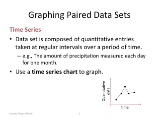
Graphing Paired Data Sets Time Series • Data set is composed of quantitative entries taken at regular intervals over a period of time. • e.g., The amount of precipitation measured each day for one month. • Use a time series chart to graph. Quantitative data time Larson/Farber 4th ed.
Example: Constructing a Time Series Chart The table lists the number of cellular telephone subscribers (in millions) for the years 1995 through 2005. Construct a time series chart for the number of cellular subscribers. (Source: Cellular Telecommunication & Internet Association) Larson/Farber 4th ed.
Solution: Constructing a Time Series Chart • Let the horizontal axis represent the years. • Let the vertical axis represent the number of subscribers (in millions). • Plot the paired data and connect them with line segments. Larson/Farber 4th ed.
Solution: Constructing a Time Series Chart The graph shows that the number of subscribers has been increasing since 1995, with greater increases recently. Larson/Farber 4th ed.
Graphs of Frequency Distributions Frequency Polygon • A line graph that emphasizes the continuous change in frequencies. frequency data values Larson/Farber 4th ed.
Example: Frequency Polygon Construct a frequency polygon for the Internet usage frequency distribution. Larson/Farber 4th ed.
Solution: Frequency Polygon The graph should begin and end on the horizontal axis, so extend the left side to one class width before the first class midpoint and extend the right side to one class width after the last class midpoint. You can see that the frequency of subscribers increases up to 36.5 minutes and then decreases. Larson/Farber 4th ed.
Graphs of Frequency Distributions Cumulative Frequency Graph or Ogive • A line graph that displays the cumulative frequency of each class at its upper class boundary. • The upper boundaries are marked on the horizontal axis. • The cumulative frequencies are marked on the vertical axis. cumulative frequency data values Larson/Farber 4th ed.
Constructing an Ogive • Construct a frequency distribution that includes cumulative frequencies as one of the columns. • Specify the horizontal and vertical scales. • The horizontal scale consists of the upper class boundaries. • The vertical scale measures cumulative frequencies. • Plot points that represent the upper class boundaries and their corresponding cumulative frequencies. Larson/Farber 4th ed.
Constructing an Ogive • Connect the points in order from left to right. • The graph should start at the lower boundary of the first class (cumulative frequency is zero) and should end at the upper boundary of the last class (cumulative frequency is equal to the sample size). Larson/Farber 4th ed.
Example: Ogive Construct an ogive for the Internet usage frequency distribution. Larson/Farber 4th ed.
Solution: Ogive 6.5 18.5 30.5 42.5 54.5 66.5 78.5 90.5 From the ogive, you can see that about 40 subscribers spent 60 minutes or less online during their last session. The greatest increase in usage occurs between 30.5 minutes and 42.5 minutes. Larson/Farber 4th ed.