Download
1 / 16
160 likes | 302 Views
The Hardy- Weinberg Hypothesis. A method of quantifying stability and change in a population. The Hypothesis. A population will remain stable unless some factor causes it to change, so we can assume “genetic equilibrium” in populations that

E N D
The Hardy-Weinberg Hypothesis A method of quantifying stability and change in a population
The Hypothesis • A population will remain stable unless some factor causes it to change, so we can assume “genetic equilibrium” in populations that • Do not have mutations adding new alleles to the gene pool • Mate randomly (no sexual selection) • Are sufficiently large to minimize the effects of random events (no genetic drift) • Are not being subjected to natural selection with regard to the traits being studied • Are not gaining or losing alleles due to migration (no gene flow)
Mutations • Mutations introduce new alleles into the gene pool which will alter the statistical evaluation of allele frequencies • The addition of mutant alleles creates the opportunity for selection (natural or sexual) that hadn’t existed before • The frequency of the mutant allele will initially be very small, and so will be more susceptible to the effects of any random events
Sexual Selection • Non-random mating with regard to a trait will be reflected in future generations • Alleles which increase the likelihood of successful mating will tend to increase in frequency in future populations • Alleles which are selected against by mate choice will decrease in frequency
Natural Selection • Any allele which confers a survival advantage will be selected for • Higher survival rates will tend to create more breeding opportunities • Higher rates of reproduction will result in more offspring, which will inherit the alleles that created that advantage • As the offspring will resemble their well adapted parents, they will also tend to survive and reproduce at relatively higher rates
Genetic Drift • Any random event will have a larger statistical influence on a small population than it would in a very large population • For example, one random death in a population of ten individuals would be a 10% change. The same random death in a population of 1000 individuals would only have a .1% effect • Small, isolated populations may evolve rapidly due to random events – basically good and bad luck
Genetic drift (part 2) • There are a few characteristic situations in which genetic drift is common: • Bottleneck effect: Some factor unrelated to the trait causes a significant population crash. Future generations will tend to resemble the survivors, even though their survival was not dependent on particular adaptations • Founder effect: Migration of a small population which becomes isolated from the main group will create a sub-population that resembles its founders.
Genetic Drift (part 3) • The populations that immediately result from a bottleneck or a migration/isolation event will necessarily be small • Smaller populations will be subjected to considerably less competition, disease, and possibly predatory pressure than larger populations – so traits that might otherwise be selected against are instead selectively neutral • Consider the ecological effects of introduced species (note zebra mussels in the great lakes and rabbits in Australia) – they experience enormous initial success in their new environment for this very reason
Gene Flow • Migration between otherwise isolated populations will have an effect on allele frequencies by adding or removing alleles • Gene flow also prevents mutations that occur in one population from remaining isolated within that population. • This concept will be very important when we consider speciation. Reproductive isolation is the foundation of evolutionary divergence and speciation
Quantifying Allele frequencies • Allele frequency is exactly what it sounds like, a measure of how frequently a particular allele appears in the gene pool – expressed as a decimal • For example, an allele with a frequency of .60 comprises 60% of the gene pool for that locus • The total of all alleles in the gene pool must logically add up to 100% (expressed as a frequency of 1.0)
Hardy-Weinberg equations • In the simplest of situations, 2 alleles exist for a trait, one dominant and one recessive. • The frequency of the dominant allele is expressed as the variable “p”, the frequency of the recessive allele is “q” • If only those 2 alleles exist, then together they make up 100% of the gene pool • p + q = 1.0
Hardy-Weinberg equations • If members of the population mate freely and randomly with regard to the trait (one of the original premises of the hypothesis), then it follows logically that the alleles already exist in every possible combination (homozygous dominant, heterozygous, and homozygous recessive) • It also follows logically that every combination of mating pairs will occur, and that the frequency of occurrence of each mating pair will reflect the frequency of the alleles
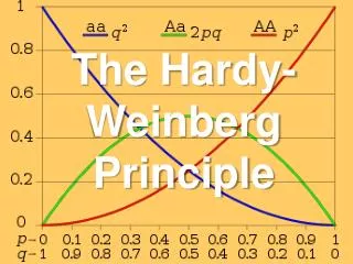
Deriving the 2nd Hardy-Weinberg equation • The 2nd Hardy-Weinberg equation is derived simply by inserting p and q into a punnett square and combining the results • p2 + 2pq + q2 = 1.0
2 equations in 2 unknowns • P2 + 2pq + q2 = 1.0, and p + q =1.0 • P2 = the frequency of homozygous dominant • 2pq = the frequency of heterozygous • q2 = the frequency of homozygous recessive • Since the homozygous recessive condition can be recognized by its phenotype, q2 is easy to calculate – it is simply the frequency of homozygous recessive individuals in the population • Once you have q2, solve for q. Once you have q, solve for p.
Sample calculation • Say a population of 100 chickens is 81% (.81) solid color and 9% (.09) grizzly. Since grizzly is recessive, q2 = .09 • The value of q is calculated as the square root of .09, so q = .3 • If q = .3, and p + q = 1.0, then p = .7 • The gene pool is 70% dominant alleles and 30% recessive alleles • We can also use these frequencies to determine the frequency of the individual genotypes using p2 + 2pq + q2 = 1.0
Applying the equations to measurable traits in the classroom • There are variations in human populations with regard to the ability to taste certain substances • We will use a blind test with a control to determine “tasting” for PTC and for Thiourea • Each student will test using filter papers designated A, B and C. One will untreated (control), one will contain a small amount of PTC and one will contain Thiourea • We will calculate the frequency of “tasters” and “nontasters” for these 2 substance and evaluate the classroom population using the Hardy-Weinberg equations