Model climate diagnostics
Model climate diagnostics. Linus Magnusson, Mark Rodwell Acknowledgement: Thomas Jung. Why do we need to monitor the model climate and model variability?. Comparison between System 3 and System 4. 1981-2010, 11 members System 3 = model cycle 31r1, T159, 62 levels

Model climate diagnostics
E N D
Presentation Transcript
Model climate diagnostics Linus Magnusson, Mark Rodwell Acknowledgement: Thomas Jung
Why do we need to monitor the model climate and model variability?
Comparison between System 3 and System 4 • 1981-2010, 11 members • System 3 = model cycle 31r1, T159, 62 levels • System 4 = model cycle 36r4,T255, 91 levels • Coupled simulations • Major model changes include • New ocean model (NEMO) • New land-surface module • New convection scheme • New cloud scheme • Change in vertical diffusion • …
Diagnostic toolbox for model climate Cryosphere(sea-ice, snowdepth) Mean on pressure levels (Z, T, U, Div) Zonal average (T, U, V, div) Seasonal mean (many parameters) Seasonal mean - independent data Mean Precip GPCP T2m vs. CRU Climate for Seasonal Forecasts Mean Climate for each model cycle Variability Activity Inter-annual variability Madden-Julian Oscillation Blocking Index Blocking 2D EOF analysis Rossby wave source Pressure index (SOI, NAO) Teleconnections Spectra Tropical waves Tropical cyclones
Zonal average temperature bias (DJF) Sys3-ERA Interim Sys4-ERA Interim
Temperature biases (cont.) Sys3-ERA Interim Sys4-ERA Interim 925 hPa Temperature bias Sea-surface temperature bias
925 hPazonal wind (DJF) Sys3-ERA Interim Sys4-ERA Interim
Precipitation bias (DJF) Sys3-GPCP Sys4-GPCP
TOA long-wave radiation (compared with CERES) Sys3-CERES Sys4-CERES ERA Interim-CERES
Blocking indexTribaldi and Molteni (1990) dz/dlat< -5 (North) dz/dlat > 0 (South)
Blocking cont. Episodes lasting >10 days Episodes lasting >1 day Sys3 (red) Sys4 (blue) ERA Int (black)
Madden-Julian oscillation Sys3 (red) Sys4 (blue) ERA Int (black)
Inter-annual variability (u-wind at 10 hPa – e.g. QBO) Sys3 Sys4 ERA Interim
Teleconnections – linear regression T2m in a grid point y=ax+b Nino3.4 SST (190E-240E,10N-10S) (logarithmic scale) Example for seasonal for Nino3.4
Teleconnection linear regression Nino3.4 SST -> z500 System 3 System 4 ERA Interim
Teleconnections - composites +/- 0.5 stdev Negative composite Positive composite
Composite on positive u10 hPa (QBO) events -> z500 System 3 System 4 ERA Interim u10 interannual variability ERA interim
Model climate for each new model cycle • For every model cycle the following configuration is run: • T255 • 3 ensemble members • 7 month integrations starting in November and May • 1981-2010 • Observed SST and coupled model
Feel free to explore the effect of the coming model cycle! http://intra.ecmwf.int/plots/d/inspect/_dir_diagnostics/Diagnostics/Climate2/ Major changes for cy38r2: Change in vertical resolution (91 -> 137 levels) Changes in the physics package