Download
1 / 13
150 likes | 377 Views
Post-process software. Diagnostics of CESM Model NCL. Wen-Ien Yu. Diagnostics of CESM Model. CICE. CAM. POP2.

E N D
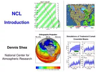
Post-process software • Diagnostics of CESM Model • NCL Wen-Ien Yu
Diagnostics of CESM Model CICE CAM POP2
The diagnostics package produces over 600 postscript plots and tables in a variety of formats from CESM (CCSM) monthly netcdf files. Climatological means for DJF, JJA, and ANN are used. The diagnostics package can be used to compare two model simulationsor for comparing a model simulation to the observational and reanalysis data. Model output on gaussian or fixed grids can be used. The code has been tested on gaussian T31, T42, T85 and T170 grids and on fixed lat/lon grids. The diagnostics package is written completely in NCL (NCAR Command Language).
cam3_5_50_s01 vs cam3_5_49_s01 1996-2005 DJF Mean Surface Pressure cam3_5_50_s01 vs NCEP Reanalysis 1996-2005 DJF Mean Zonal wind
cam3_5_50_s01 vs cam3_5_49_s01 Annual implied northward ocean heat transport cam3_5_50_s01 vs cam3_5_49_s01 1996-2005 200mb zonal wind
CESM Post-Processing Utilities: http://www.cesm.ucar.edu/models/cesm1.0/model_diagnostics/ Registration: (if you don’t have NCAR, NERSC, or NCSS account) http://www.cgd.ucar.edu/amp/amwg/diagnostics/code.html CAM: http://www.cesm.ucar.edu/models/cesm1.0/register/register_cesm1.0.cgi
140.112.66.145 /home/comet/DIAGNOSTICS/ NCO: http://nco.sourceforge.net/ The netCDF Operators, or NCO, are a suite of programs known as operators. The operators facilitate manipulation and analysis of data stored in the self-describing netCDF format. Each NCO operator (e.g., ncks) takes netCDF input file(s), performs an operation (e.g., averaging, hyperslabbing, or renaming), and outputs a processed netCDF file.
NCAR CommandLanguage NCL, a product of the Computational & Information Systems Laboratory at the National Center for Atmospheric Research (NCAR), is a free interpreted language designed specifically for scientific data processing and visualization. Numerous analysis functions are built-in NCL. NCL has robust file input and output. It can read and write netCDF-3, netCDF-4 classic , HDF4, binary, and ASCII data, and read HDF-EOS2,HDF-EOS5, GRIB1,GRIB2and OGR files (shapefile, MapInfo, GMT, TIGER) . Overview: http://www.ncl.ucar.edu/get_started.shtml Getting Started: http://www.ncl.ucar.edu/get_started.shtml Examples: http://www.ncl.ucar.edu/Applications/ Functions: http://www.ncl.ucar.edu/Document/Functions/
Stream Function from U, V netCDFfiles ; Calculate 200mb daily Stream Functkon begin ; load netcdf data in = addfile("/home/comet/NOAA_NCEP_NCAR/v_daily/vwnd.1983_1989.nc","r") in2 = addfile("/home/comet/NOAA_NCEP_NCAR/u_daily/uwnd.1983_1989.nc","r") nlat = 73 nlon = 144 ntim = 2557 ; 1990-2008: 6940 days v=in->vwnd u=in2->uwnd lon=in->lon lat=in->lat level=in->level time=in->time uvmsg = 1e+36 ; missing value of psi and vp matrix psi = new ( (/ntim,nlat,nlon /), float, uvmsg ) ; stream function vp = new ( (/ntim,nlat,nlon /), float, uvmsg ) ; velocity potential ; u, v => psi do i=0,ntim-1,1 uv2sfvpg (u@scale_factor*u(i,10,:,:)+u@add_offset,v@scale_factor*v(i,10,:,:)+v@add_offset,psi(i,:,:),vp(i,:,:)) ; form NCL website Functions end do ; output netcdf data system("/bin/rm -f /home/comet/NOAA_NCEP_NCAR/200psi.day.1983_1989.nc") ncdf = addfile("/home/comet/NOAA_NCEP_NCAR/200psi.day.1983_1989.nc" ,"c") ncdf->lon=lon ncdf->lat=lat ncdf->time=time psi!0 = "time" psi!1 = "lat" psi!2 = "lon" psi&time = time psi&lat = lat psi&lon = lon psi@long_name = "200hPa Stream Function" ncdf->psi=psi end PS: For 14(supermic)and15(GPU), please add export NCARG_ROOT=/usr/local/ & export NCARG_ROOT= /opt/ncl_ncarg520.intel_11/ respectively in ~/.bashrc .
; NCL Graphics Example load "$NCARG_ROOT/lib/ncarg/nclscripts/csm/gsn_code.ncl" load "$NCARG_ROOT/lib/ncarg/nclscripts/csm/gsn_csm.ncl" begin in = addfile("/home/comet/NOAA_NCEP_NCAR/200psi.day.1983_1989.nc","r") psi = in->psi wks = gsn_open_wks("ps","example") ; open a workstation to draw graphics gsn_define_colormap (wks,"BlAqGrYeOrRe") ; choose colormap res = True ; plot mods desired res@cnFillOn = True ; turn on color res@cnLinesOn = False ; no contour lines res@gsnSpreadColors = True ; use full color map res@lbBoxLinesOn = False ; turn off box between colors res@lbLabelAutoStride= True res@cnLabelDrawOrder= "PostDraw" ; draw lables over lines res@cnLevelSelectionMode= "ManualLevels" ; manual levels res@cnMinLevelValF= -1.25e+08 res@cnMaxLevelValF = 0 ; 1.2e+08 res@cnLevelSpacingF = 1e+07 res@pmTickMarkDisplayMode = "Always" ; turn on tick marks res@mpProjection = "Satellite" ; choose map projection res@mpCenterLonF = 150.0 ; choose center lon res@mpCenterLatF = 30; choose center lat res@mpSatelliteDistF = 3.0 ; choose satellite view res@mpOutlineOn = True ; turn on continental outlines res@mpGridAndLimbOn= True ; turn on lat/lon lines res@tiMainString = "Stream Function Decenber 1st, 1983" ; add title res@sfXCStartV = min(psi&lon) ; where to start x res@sfXCEndV = max(psi&lon) ; where to end x etc res@sfYCStartV = min(psi&lat) res@sfYCEndV = max(psi&lat) map = gsn_csm_contour_map(wks,psi(0,:,:),res) end PlotingnetCDF file