SHEAR STRESS
SHEAR STRESS. A. M. Artoli 1 , D. Kandhai 2 , H.G. Hoefsloot 3 , A.G. Hoekstra 1 and P.M.A. Sloot 1. Shear stress plays a dominant role in biomechanical deseases related to blood flow problems. . IN LATTICE BOLTZMANN. Motivation. Aorta with a bypass.


SHEAR STRESS
E N D
Presentation Transcript
SHEAR STRESS A. M. Artoli1 , D. Kandhai2, H.G. Hoefsloot3, A.G. Hoekstra1 and P.M.A. Sloot1
Shear stress plays a dominant role in biomechanical deseases related to blood flow problems. IN LATTICE BOLTZMANN Motivation Aorta with a bypass
Conventionally, the shear stress is calculated from the computed gradients of velocity profiles obtained from experimental or simulation models. SIMULATIONS
Why LBM? • Recently, the Lattice Boltzmann Method (LBM) has attracted much attention in simulations of complex fluid flow problems for its simple implementation and inherent parallelism. • The LBM can be used to calculate the local components of the stress tensor in fluid flows WITHOUT a need to estimate velocity gradients. This has two benefits over conventional CFD methods : Increasing accuracy and decreasing computational cost.
Definition • The stress tensor is defined as[1] [1] L.Landau and E. Lifshitz, Fluid mechanics, Pergamon Press (1959).
The LBM • The LBM is a first order finite difference discretization of the Boltzmann Equation that describes the dynamics of continuous particle distribution function which is the probability of finding a particle with microscopic velocity • The velocity is descritized into a set of vectors ei • The inter-particle interactions are contained in the collision term W • The resulting Lattice Boltzmann Equation is: • The collision term is simplified to the linear case via the single time relaxation Approximation (STRA);
Theory • The equilibrium distribution is given by where wi = 4/9 for the rest particle, 1/9 for particles moving in x and y directions and 1/36 for diagonal ones. Also, Conservation laws are satisfied : • mass • momentum
Theory , cont. • The LB equation is then discretized in space and time to yield • Using the multi-scale Chapman expansion of the kinetic moments of the distribution functions, the macroscopic NS equation can be derived in the limit of low Mach number (u << Cs=; the speed of sound). Where is the pressure. The kinematic viscosity and the equation of state are given by
The stress tensor in LBM The stress tensor for a 9 particles 2D LBM model is given by [2] where is the dissipative part of the momentum tensor , which can be obtained during the collision operation, without a need to take the derivatives [2] S. Hou, S. Chen, g. Doolen and A. Cogley. J.Comp.Phys. 118, 329 (1995).
How the stress tensor is computed? • Select a model (e.g:D2Q9) • For All nodes{ • compute the density and velocity from the fi’s • initialize sab with 0 • for all directions{ • . sab += c[k]a c[k]bDf (1-1/(2t)) -r cs2dab. • Collide: fab [k] = fab[k]-(fab[k]- fabeq[k])/t } }
BENCHMARK-1 • Plane Poiseulle steady flow Analytic solutions:
BENCHMARK-2 Couette Flow with injection upper wall moves with hrizontal velocity Un Lower veocity is fixed Vertical injection with speed U0 Analytic solutions
BENCHMARK-3 Symmetric Bifurcation
Ongoing Research • 2D oscillatory Poiseuille flow • a =3.07 • error ~ 10-2 for integer time steps and ~10-15 for half-time steps. • shown: Full-period analytic solutions (lines) and simulation results (points)
Womersley solution • 3D Preliminary Results • error ~ for integer time steps and ~ for half-time steps. • shown: Full-period Analytic solutions (lines) and simulation results (points)
Conclusions • With LBM, the shear stress can be obtained from the distribution functions without a need to compute derivatives of velocity profiles. • LBM is second order accurate in space and time. • Pulsatile shear stress can still yield accurate results.
Flow characteristics • There is a Phase lag between the pressure and the fluid motion. • At low a, steady Poiseuille flow is obtained. • At high a, we have the annular effect: • Profiles are flattened • The phase lag increases toward the center. • The shear stress is very low near the center and reasonably high at the walls.
Simulations • Flow is driven by a time dependent body force P = A sin(w t) in the x-direction. A= initial Magnitude of P, w= angular frequency, t= simulation time . • Boundary conditions • inlet and outlet: Periodic boundaries. • Walls: bounce-Back • Parameters • a ranges from 1-15 • t = 1 • Grid size : • 2D : 10 x50 for a = and 20 x100 for a= • 3D : 50 x 50 x 100
Results, Continued • a = • error ~ 10-2 for integer time steps and ~ 10-15 for half-time steps. • shown: Full-period Analytic solutions (lines) and simulation results (points)