Download
1 / 76
770 likes | 980 Views
Animal Communication. Part 2: Functional Issues. III. Function, b. Information & Decisions. Question posed by female: Is this male healthy or sick? Signals assigned to the same question are a signal set (e.g. in this example, both song & dance signal health)

E N D
Animal Communication Part 2: Functional Issues
III. Function, b. Information & Decisions • Question posed by female: Is this male healthy or sick? • Signals assigned to the same question are a signal set • (e.g. in this example, both song & dance signal health) • Alternative answers: male is healthy; male is sick….these are the conditions • Sender has a code that correlates the signal with the conditions: • Songs are fast in healthy males, slow in sick males • Dance is vigorous in healthy males, not in sick males • All signals pooled across all questions and signal sets is the signal repertoire; size depends on the number of questions asked and the number of possible answers
III. Function, b. Information & Decisions Example: Territorial defense QUESTIONS ALTERNATIVE ALTERNATIVE CONDITIONS SIGNALS
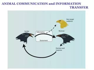
III. Function, b. Information & Decisions • There are two basic kinds of information that can be transferred by signals: • Confirmation of Conditions: Signals confirm which of several alternatives suspected by the Receiver is currently true • Novel Facts: Signals are used to share some fact unsuspected by the Receiver
III. Function, b. Information & Decisions • Two kinds of information can be transferred by signals: • Communication by most animals is of the second type of Scenario: receivers “know” the likely alternatives, either through learning or genetic biases or both, and signals largely serve to confirm which among these alternatives is currently true • Where novel alternatives do turn up, these are usually assigned to one of the existing alternatives (e.g. one more type of predator)
III. Function, b. Info & Decisions1. Information as Probabilities • Information as Probabilities: • If the alternatives to some question are already known, then what must change with the provision of information are the relative probabilities that each alternative might be true • We say the probabilities are updated with the provision of information For example, you may start your day estimating a 1x10⁻⁵ % chance of being killed by a terrorist attack, but increase that to 1.1x10⁻⁵ % after seeing the “orange” DHS alert
III. Function, b. Info & Decisions1. Information as Probabilities • Information as Probabilities: • So today we’ll be talking about how receivers use information encoded in signals to update their estimated probabilities that certain conditions are true, and thereby make decisions • These decisions determine the benefits that both receivers and sender gain by communicating
C1 Probability III. Function, b. Info & Decisions1. Information as Probabilities Example: The receiver (you) want to know whether you are going to like the new movie by a favorite director Your priors are the percentage of movies by that director that you previously liked (72%) When you read a positive movie review in the paper (the signal), you update your probability estimates with this new information… How do you update your estimate? 1- Pprior Pprior = 0.72 1- Pupdated Pupdated = ?? C2 Probability C1 Probability C2 Probability C1 = Love it C2 = Hate it
III. Function, b. Info & Decisions1. Information as Probabilities The reliability of signals can be mapped on a coding matrix A perfect signal is never wrong When it is received, one needle goes to 1.0 probability and the other to 0: Condition: C1 C1 C2 S1 Signal: S2 1- Pupdated Pupdated = 1.0 C1 Probability C2 Probability C1 = Love it C2 = Hate it
III. Function, b. Info & Decisions1. Information as Probabilities • An imperfect signal is only correct some fraction X% of the time • Each signal moves the needles only part way towards 0 or 1 • This is much more common in animal communication Condition: C1 C1 C2 S1 Signal: S2 C1 Probability C2 Probability C1 = Love it C2 = Hate it
III. Function, b. Info & Decisions1. Information as Probabilities Imperfect Signals: If you read more movie reviews, each gives new information, but each has a smaller effect on your opinion (diminishing returns to continued reading of reviews) C1 Probability C2 Probability C1 = Love it C2 = Hate it
III. Function, b. Info & Decisions2. The Amount of Information • Since the change in probabilities with receipt of a given signal depends on the prior probability, we need to take prior probabilities into account when we measure the amount of information the signal provides to the Receiver • So we use the base 2 logarithm of the ratio of updated to prior probability estimates.Why? • We use logarithms because they give the same absolute value regardless of which direction the estimate changes, with a sign indicating the direction: • e.g. log2(0.9/0.1) = 3.17 and log2(0.1/0.9) = –3.17 • Why do we use base 2 logs?
III. Function, b. Info & Decisions2. The Amount of Information • It is easiest to think of information as the answers to specific questions • Binary Questions: The simplest type of question has only two possible answers: yes or no, A or B, male or female, etc. • Complex Questions: Any complex question with a finite number of possible answers can be broken down into a series of binary questions
III. Function, b. Info & Decisions2. The Amount of Information • E.g. Cuckoo Eggs: One egg in the nest is a cuckoo egg. How many binary questions do you have to ask to find it?
III. Function, b. Info & Decisions2. The Amount of Information • General Case: If M is the number of alternative answers to a complex question, and H is the number of binary questions that need to be asked to find which alternative is true, then • M = 2H • One bit is the information required to answer a binary question • It takes H bits to answer a question with M alternative answers
III. Function, b. Info & Decisions2. The Amount of Information • General Case: If M = 2H, then if follows that • H = log2 M • WhereH is the number of bits to answer a question, and M is the number of alternative answers (conditions) • ...you can compute log2 M on your calculator without using base 2 logs by calculating ln(M)/ln(2) or log10M/log102 • ...a value of M that is not an integer power of 2 is OK: thus log23 = 1.58
III. Function, b. Info & Decisions2. The Amount of Information • So that’s how we quantify information; how does this relate to probability estimates? • As you saw before, we measure the amount of information the signal provides to the Receiver as the base 2 logarithm of the ratio of updated to prior probability estimates • Now, we formalize that in an equation: • The amount of information in bits transferred by a signal about the likelihood of a particular answer A to a question
III. Function, b. Info & Decisions2. The Amount of Information • Perfect Signals: After receipt of a perfect signal, the numerator in the amount of information expression, P(A)updated goes to either 0 or 1 • If A is the answer that is now known to be true, the amount of information provided by the signal about A is • HT = log2(1/P(A)prior) = – log2(P(A)prior)
I. What is Information? B. The Amount of Information If you have these priors (P0) for the 5 possible moods of your dog: Wants to play: 0.2 Wants food: 0.4 Amorous: 0.2 Fearful: 0.1 Aggressive: 0.1 If you receive a “play signal”, which is a perfect signal, how much information does it give you? HT play signal =
III. Function, b. Info & Decisions2. The Amount of Information • Imperfect Signals: P(A)updated never goes to 1.0 after receipt of an imperfect signal. Instead, we are left with • which can be rewritten as • Which is the same as • HT = Hprior – Hupdated
III. Function, b. Info & Decisions2. The Amount of Information • H as uncertainty: HT = Hprior – Hupdated • The first term, Hprior = –log2(P(A)prior), is the amount of information in bits required to remove ALL of our prior uncertainty about whether A was true before the signal • The 2nd term, Hupdated = –log2(P(A)updated), is the amount of information in bits required to remove ALL uncertainty about whether A is true after receipt of the signal • The difference between these two terms, HT, is the amount of initial uncertainty about whether A was true that was removed by the signal • It is the amount of information transferred through communication
III. Function, b. Info & Decisions2. The Amount of Information • Example: Suppose P(A)prior = 0.5 • how does HTchange with different values of P(A)updated?
III. Function, b. Info & Decisions2. The Amount of Information • Information theory was developed by Claude Shannon to find fundamental limits on compressing and reliably storing and communicating data • Shannon entropy is a measure of the uncertainty associated with a random variable; quantifies the info contained in a message (in bits). • How is information theory used?We aren’t usually privy to what animals are trying to say...how many options are available, their priors are, etc. • So while conceptually useful, the classic information theory we just learned is difficult to apply directly in animal communication. Many statistics have been built on this foundation, however, which are also conceptually useful, and more tractable to use • Markov Chain Models of syntax are one example. Signal Detection Theory is an information-theoretic framework, which uses a statistical approach, similar to Type I and Type II errors in statistics (Wiley, Adv. Study Behav. 2006).
III. Function, a. Info & Decisions2. The Amount of Information • Signal Detection Theory (Acoustics) • Each curve is a probability density function (PDF) of for the outputs of a perceptual channel with and w/out the signal; The threshold is where response occurs • Signal detection theory predicts how animals should increase the separation of the background vs. signal+background PDFs (i.e. signal-to-noise ratio), e.g.: • Increase repetition rate • Use diff freqs than background • Use diff amplitude modulation • Use longer signals
III. Function, b. Info & Decisions2. The Amount of Information • Another example of how information theory is used: • Zipf’s statistic evaluates the signal composition or ‘structure’ of a repertoire by examining the frequency of use of signals in relationship to their ranks (i.e. first, second, third versus most-to-least frequent)(McCowan, et al. 1999) • Measures the potential capacity for info transfer at the repertoire level by examining the ‘optimal’ amount of diversity and redundancy necessary for communication transfer across a ‘noisy’ channel (i.e. all complex audio signals will require some redundancy) <1mo. old dolphin whistles Adult dolphin whistles Log10 Frequency Log10 Rank of use
III. Function, b. Info & Decisions3. Encoding Information • Now we’ll discuss how the ideal receiver uses information to update his/her probability estimates (i.e. calculate pupdated) • Example: Suppose the Receiver needs to know whether condition C1 or condition C2 is currently true • There are two signals, S1 and S2 that can be used to provide information about this question • We can summarize the coding rules for this system by constructing a coding matrix with the conditional probabilities in the cells Condition: C1 C2 E.g. conditional probability P(S1|C1)is the probability that signal 1 occurs when condition 1 is true P(S1|C1) P(S1|C2) S1 Signal: S2 P(S2|C1) P(S2|C2)
III. Function, b. Info & Decisions4. Making Decisions • A Receiver’s task is to combine prior probabilities, knowledge of the coding matrix, and receipt of a particular signal to produce new updated probabilities of the alternatives • There are many ways to update, but no mechanism of updating can be more accurate than Bayesian updating; it’s the theoretical upper limit
III. Function, b. Info & Decisions4. Making Decisions, i. Bayesian Updating • Basic Logic: First, assemble the priors and coding matrix • Baye’s Theorem states that the updated probability that C1 is true after receipt of signal S1 is: C1 C2 Condition: Note that all the numbers we need to solve this are in our coding matrix S1 Signal: S2 p(C1) p(C2) Priors:
III. Function, b. Info & Decisions4. Making Decisions, i. Bayesian Updating The numerator is the prob that we would see C1 and S1 together The denominator is the prob that we would see C1 and S1 together plus the prob we would see S1 and C2 together; thus the denominator is the overall fraction of time we might see an S1 signal The best estimate of the updated probability is thus the fraction of time that we observe an S1 signal and it co-occurs with C1
III. Function, b. Info & Decisions4. Making Decisions, i. Bayesian Updating • Example: • Suppose females of a bird species use the rate of male songs to assess the health of potential mates • Healthy males tend to sing Fast songs and sick ones tend to sing Slow songs • Suppose the two types of males are almost equally common (52% healthy, 48% sick) • Suppose also that coding is not perfect: Good males sing Fast songs 70% of the time, whereas Bad males sing Slow songs 60% of the time
III. Function, b. Info & Decisions4. Making Decisions, i. Bayesian Updating • Example: We first assemble the information available before receipt of a signal • A female assumes any male has a 52% chance of being Good before she hears any songs Condition: Good Bad Fast 0.70 0.40 Signal: Probability Good Slow 0.30 0.60 Priors: 0.52 0.48
III. Function, b. Info & Decisions4. Making Decisions, i. Bayesian Updating • Example: After receipt of a Fast song, that estimate goes to: • …If that song had been Slow, her estimate would have been: Condition: Good Bad Fast 0.70 0.40 Signal: Probability Good Slow 0.30 0.60 Priors: 0.52 0.48
III. Function, b. Info & Decisions4. Making Decisions, i. Bayesian Updating • Example: After receipt of a Fast song, that estimate goes to: Sequential updating: If the female is finished listening, then 0.655 is her final estimate. But if she’s going to keep listening, she now updates her priors to the new values she has obtained Condition: Good Bad 1.00 Fast 0.70 0.40 p(Good) Signal: Slow 0.30 0.60 0.5 # Songs Sampled Priors: 0.52 0.48
III. Function, b. Info & Decisions4. Making Decisions, i. Bayesian Updating • Example: Suppose 2nd song is also Fast: And she again updates her priors by replacing them with the most recent updated probabilities Condition: Good Bad 1.00 Fast 0.70 0.40 p(Good) Signal: Slow 0.30 0.60 0.5 # Songs Sampled Priors: 0.655 0.345
III. Function, b. Info & Decisions4. Making Decisions, i. Bayesian Updating • Example: Suppose 3nd song is Slow: She updates to the new probabilities and uses these as the next prior probabilities… Condition: Good Bad 1.00 Fast 0.70 0.40 p(Good) Signal: Slow 0.30 0.60 0.5 # Songs Sampled Priors: 0.766 0.234 0.621 0.379
III. Function, b. Info & Decisions4. Making Decisions, i. Bayesian Updating • Example: Suppose 4th song is Fast: And so on… Condition: Good Bad 1.00 Fast 0.70 0.40 p(Good) Signal: Slow 0.30 0.60 0.5 # Songs Sampled Priors: 0.621 0.379
III. Function, b. Info & Decisions4. Making Decisions, i. Bayesian Updating • Example: Sequential Sampling: Although the trajectory is jagged (and different every time), the general trend if a male is truly Good will be up, and if he is Bad, down. The Truth will come out…. 1.00 Good Male Trajectory Fast Songs p(Good) 0.5 Slow Songs Bad Male Trajectory 0.0 # Songs Sampled
III. Function, b. Info & Decisions4. Making Decisions, i. Bayesian Updating • Example: Sequential Sampling: Note that in general, the change in probabilities, Dp, for each successive song is smaller than for earlier songs • What does this mean for the amount of information transmitted? 1.00 p(Good) 0.5 0.0 # Songs Sampled
III. Function, b. Info & Decisions4. Making Decisions, i. Bayesian Updating • Example: Sequential Sampling: Finally, note that less accurate coding matrices will cause the cumulative estimate to take longer to asymptote to the extreme: • What does this mean for the amount of information transmitted? 1.00 More accurate code Less accurate code p(Good) 0.5 0.0 # Songs Sampled
III. Function, b. Info & Decisions4. Making Decisions, i. Bayesian Updating • Do Animals use Bayesian updating? • Sequential assessment of signals and cues is very common, from primates to honeybees; Bayesian updating is an optimal strategy for sequential updating if: • Animals have reasonable prior probabilities about likelihood of alternative conditions, and accuracy of coding scheme • Animals have time to assess signals and cues sequentially • Animals have the neural capacity to store the information • Some animals use short cuts and rules of thumb for updating which may be quite good. Bayesian updating is the best possible, but that’s not always the optimal thing to do… Even so, understanding BU is important because it defines the upper limit of what’s possible for comparison!
III. Function, b. Info & Decisions4. Making Decisions, i. Bayesian Updating • Mate searching by female satin bowerbirds: Females visit males at their bowers to assess their signals (bower, decs) Males mate with multiple females How should females find the best male? Alternative hypotheses: Threshold vs. Best-of-n models Al Uy found that females visit multiple males at their bowers during the mating season and they visit each male multiple times (sequential updating) before mating with one male Fits predictions of a Best-of-n model with Bayesian updating (Luttbeg 1996)
III. Function, b. Info & Decisions4. Making Decisions, i. Bayesian Updating • Mate searching by female satin bowerbirds: When females find a high-quality male, they shop less the next year and often mate with him again (they re-affirm prior estimates and re-mate if he’s still good) Females who mated with a bad male, will avoid him the following year and find a better mate Older (more experienced) females often went straight back to the best male in the population each year without shopping When he died, they were all forced to start shopping again… (Uy et al. 200, 2001)
III. Function, b. Info & Decisions5. Take Home Messages • Benefits of Communication: • Animals know the potential answers to most questions but may be unsure which answer is currently true • Senders can provide information that helps Receivers improve their probability estimates for each alternative • Receivers can improve estimates further by sampling successively and/or only attending to accurate signals • Costs of Communication: • Providing more accurate signals or sampling successively increases the costs of communication for both parties • How far does an imperfect signal have to change a prior probability before it is worth the costs of sending and receiving it? This is an optimization problem
III. Function, b. Info & Decisions5. Take Home Messages • Optimal Information: • It never really pays to try to send or seek perfect information through signals • Instead, animals are likely to establish some intermediate compromise in which they sometimes err • Errors in communication are not evidence of faulty evolution but the reasonable application of good economics • Optimality ≠ perfection!
III. Function, c. Honesty in Advertising • Early ethological approach:Because signals evolve from intentions, preparatory movements, physiological precursors, etc… they reliably predict what sender will do next because sender can’t help it (they are constrained to be honest). Often ignored conflict entirely, and viewed communication as an altruistic exchange of information • Dawkins/Krebs arms race and early game models:Senders should try to trick, mislead, and manipulate receivers into giving responses benefiting sender, and receivers should become mind-readers trying to discount false signals • Zahavi Handicaps:Receivers only pay attention to signals that impose a cost (handicap) on senders, which makes it costly to send dishonest or exaggerated signals
III. Function, c. Honesty in Advertising,2. Current Thinking There are several dozen game-theoretic models of communication when there is a conflict of interest between the sender and receiver, each depicting a different signaling context Common theme: There must be some type of cost or constraint imposed on senders to guarantee honesty, but this cost is different for each model or context • We’ll discuss 3 categories of costs in communication: • A. Necessary costs • B. Incidental costs • C. Constraints Both senders and receiver may pay these costs, but it is the cost to the senders which we use to categorize the signals. Costs to receivers are also important, because they select for “mind-readers” who only respond to honest signals.
III. Function, c. Honesty in Advertising,1. Costs A. Necessary Costs: Costs paid up front, do not depend on receiver response, includes: • Prior investment by sender in special structures, coloration, organs, brain circuitry, etc. • Immediate costs sustained by sender while communicating such as time lost, energetic expenditure, and predation risk • Receivers also pay some necessary costs (assessment costs, possible brain and sensory costs, etc.), which favors receivers who only pay attention to honest signals (i.e. “mind-readers”).
III. Function, c. Honesty in Advertising,1. Costs B. Incidental Costs: Decreases in magnitude of payoffs to either the sender or receiver; does depend on receiver response • Costs to the sender: if the receiver punishes the sender for sending the signal (e.g. badges of status), this selects for honest signals. • Receivers can also pay incidental costs: If sender deceives the receiver into acting against the receiver’s interests (sender deceit, bluff, exaggeration, withholding information). These costs select for receivers who only pay attention to honest signals (i.e. “mind-readers”).
III. Function, c. Honesty in Advertising,1. Costs • C. Constraints: limits on communication imposed by environment, phylogenetic history and physics • Examples: Frequency and amplitude are limited by body size, brain size limits learning of songs, etc. • These aren’t always costly to signalers, but they prevent cheating because overcoming the constraints (if that’s even possible), would require costs too large to bear