The Block Diagram
Block diagram is a graphical tool to visualize the model of a system and evaluate the mathematical relationships between its components, using their transfer functions.

The Block Diagram
E N D
Presentation Transcript
Block diagram is a graphical tool to visualize the model of a system and evaluate the mathematical relationships between its components, using their transfer functions. In many control systems, the system equations can be written so that their components do not interact except by havingthe input of one part be the output of another part. The transfer function of each components is placed in a box, and the input-output relationships between components are indicated by lines and arrows. Chapter 3 Dynamic Response The Block Diagram
Chapter 3 Dynamic Response The Block Diagram • Using block diagram, the system equations can be simplified graphically, which is often easier and more informative than algebraic manipulation.
Chapter 3 Dynamic Response Elementary Block Diagrams Blocks in series Blocks in parallel with their outputs added Pickoff point Summing point
Chapter 3 Dynamic Response Elementary Block Diagrams Single loopnegative feedback Negativefeedback ? What about single loop with positive feedback?
Chapter 3 Dynamic Response Block Diagram Algebra
Chapter 3 Dynamic Response Block Diagram Algebra
Chapter 3 Dynamic Response Transfer Function from Block Diagram Example: Find the transfer function of the system shown below.
Chapter 3 Dynamic Response Transfer Function from Block Diagram Example: Find the transfer function of the system shown below.
Chapter 3 Dynamic Response Transfer Function from Block Diagram
Chapter 3 Dynamic Response Transfer Function from Block Diagram Example: Find the response of the system Y(s) to simultaneous application of the reference input R(s) and disturbance D(s). WhenD(s) =0, ? WhenR(s) =0,
Chapter 3 Dynamic Response Transfer Function from Block Diagram
The poles are the values of s for which the denominator A(s) = 0. The zeros are the values of s for which the numerator B(s) = 0. Chapter 3 Dynamic Response Definition of Pole and Zero • Consider the transfer function F(s): Numerator polynomial Denominator polynomial • The system response is given by:
When σ>0, the pole is located at s < 0, The exponential expression y(t) decays. Impulse response is stable. When σ<0, the pole is located at s > 0, The exponential expression y(t) grows with time. Impulse response is referred to as unstable. Chapter 3 Dynamic Response Effect of Pole Locations • Consider the transfer function F(s): A form of first-order transfer function • The impulse response will be an exponential function: • How?
The terms e–t and e–2t, which are stable, are determined by the poles at s = –1and –2. This is true for more complicated cases as well. In general, the response of a transfer function is determined by the locations of its poles. Chapter 3 Dynamic Response Effect of Pole Locations Example: Find the impulse response of H(s), • PFE
Chapter 3 Dynamic Response Effect of Pole Locations Time function of impulse response assosiated with the pole location in s-plane LHP RHP LHP : left half-plane RHP : right half-plane
Chapter 3 Dynamic Response Representation of a Pole in s-Domain • The position of a pole (or a zero) in s-domain is defined by its real and imaginaryparts, Re(s)andIm(s). • In rectangular coordinates, the complex poles are defined as(–s ±jωd). • Complex poles always come in conjugate pairs. A pair of complex poles
Chapter 3 Dynamic Response Representation of a Pole in s-Domain • The denominator corresponding to a complex pair will be: • On the other hand, the typical polynomial form of a second-order transfer function is: • Comparing A(s) and denominator of H(s), the correspondence between the parameters can be found: ζ : damping ratio ωn : undamped natural frequencyωd : damped frequency
Chapter 3 Dynamic Response Representation of a Pole in s-Domain • Previously, in rectangular coordinates, the complex poles are at (–s±jωd). • In polar coordinates, the poles are at (ωn, sin–1ζ), as can be examined from the figure.
Chapter 3 Dynamic Response Unit Step Resonses of Second-Order System
Chapter 3 Dynamic Response Effect of Pole Locations Example: Find the correlation between the poles and the impulse response of the following system, and further find the exact impulse response. Since The exact response can be otained from:
Chapter 3 Dynamic Response Effect of Pole Locations To find the inverse Laplace transform, the righthand side of the last equation is broken into two parts: Damped sinusoidal oscillation
Chapter 3 Dynamic Response Time Domain Specifications • Specification for a control system design often involve certain requirements associated with the step response of the system: • Delaytime, td, is the time required for the response to reach half the final value for the very first time. • Rise time, tr, is the time needed by the system to reach the vicinity of its new set point. • Settling time, ts, is the time required for the response curve to reach and stay within a range about the final value, of size specified by absolute percentage of the final value. • Overshoot, Mp, is the maximum peak value of the response measured from the final steady-state value of the response (often expressed as a percentage). • Peak time, tp, is the time required for the response to reach the first peak of the overshoot.
Chapter 3 Dynamic Response Time Domain Specifications
Chapter 3 Dynamic Response First-Order System • The step response of first-order system in typical form: is given by: • t: time constant • For first order system, Mp and tp do not apply
Chapter 3 Dynamic Response Second-Order System • The step response of second-order system in typical form: is given by:
Chapter 3 Dynamic Response Second-Order System • Time domain specification parameters apply for most second-order systems. • Exception: overdamped systems, where ζ > 1 (system response similar to first-order system). • Desirable response of a second-order system is usually acquired with 0.4 < ζ < 0.8.
Chapter 3 Dynamic Response Rise Time • The step response expression of the second order systemis now used to calculate the rise time, tr,0%–100%: • Since , this condition will be fulfilled if: φ or, tr is a function of ωd
Chapter 3 Dynamic Response Settling Time • Using the following rule: with: • The step response expression can be rewritten as: where: ts is a function of ζ
Chapter 3 Dynamic Response Settling Time • The time constant of the envelope curves shown previously is 1/ζωn, so that the settling time corresponding to a certain tolerance band may be measured in term of this time constant.
Chapter 3 Dynamic Response Peak Time • When the step response y(t) reaches its maximum value (maximum overshoot), its derivative will be zero:
Chapter 3 Dynamic Response Peak Time • At the peak time, ≡0 • Since the peak time corresponds to the first peak overshoot, tp is a function of ωd
Chapter 3 Dynamic Response Maximum Overshoot • Substituting the value of tp into the expression for y(t), if y(∞) = 1
Chapter 3 Dynamic Response Example 1: Time Domain Specifications Example: Consider a system shown below with ζ = 0.6 and ωn= 5 rad/s. Obtain the rise time, peak time, maximum overshoot, and settling time of the system when it is subjected to a unit step input. After block diagram simplification, Standard form of second-order system
Chapter 3 Dynamic Response Example 1: Time Domain Specifications In second quadrant
Chapter 3 Dynamic Response Example 1: Time Domain Specifications Check y(∞) for unit step input, if
Chapter 3 Dynamic Response Example 1: Time Domain Specifications
Chapter 3 Dynamic Response Example 2: Time Domain Specifications Example: For the unity feedback system shown below, specify the gain K of the proportional controller so that the output y(t) has an overshoot of no more than 10% in response to a unit step.
Chapter 3 Dynamic Response Example 2: Time Domain Specifications : K = 2 :K = 2.8 : K = 3
Chapter 3 Dynamic Response Homework 2 • No.1 • Obtain the overall transfer function of the system given below. + – + • No.2, FPE (6thEd.), 3.25. • Note: Verify your design using MATLAB and submit also the printout of the unit-step response. • Deadline: Thursday, 26.09.2013.