Download
1 / 21
220 likes | 442 Views
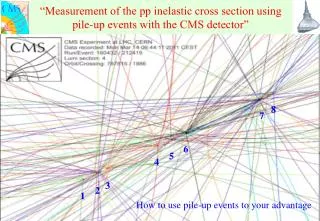
“Measurement of the pp inelastic cross section using pile-up events with the CMS detector”. 8. 7. 6. 5. 4. 3. 2. 1. How to use pile-up events to your advantage. Analysis technique. The probability of having n pileup depends only on the total s ( pp ) cross section:.

E N D
“Measurement of the pp inelastic cross section using pile-up events with the CMS detector” 8 7 6 5 4 3 2 1 How to use pile-up events to your advantage
Analysis technique • The probability of having npileup depends only on the total s(pp) cross section: (L*s)n_pileup * e –(L*s) P (nPileup) = npileup! If we count the number of pile-up events as a function of luminosity, we can measure s(pp). For an accurate measurement we need a large luminosity interval.
Steps • Acquire the bunch crossing using a primary event: • the bunch crossing is recorded because there was an event that fired the trigger. We don’t use this primary event, we only use it to record the bunch crossing • Count the number of pile-up events: • for any give bunch crossing, we count the number of vertices in the event. • Correct the number of visible vertices for various effects: • vertex merging, vertex splitting, real secondary vertices… • Fit the probability of having n = 0,….8 pile-up events as a function of luminosity: • using a Poisson fit, we obtain 9 values of s(pp)n • Fit the 9 values together: • from s(pp)n we obtain s(pp)
Luminosity and pile-up events LHC is doing really well, it has reached a record instantaneous luminosity of 1.7*1033 cm-2 s-1. However for this study the important parameter it the instantaneous luminosity per bunch (currently 1080 bunches) We studied events with: 0-8 pile-up events and luminosity range 0 - 0.7 1030 cm-2 s-1 (2010 data taking period)
How many pile-up events are there? Number of pile-up events: # vertices -1 Number of vertices We studied events with 0-8 pile-up events (non enough statistics to go further)
Vertex reconstruction The goal of the analysis is to count the number of pile-up events as a function of luminosity. This means we need to count vertices.
Vertex requirements Position along the beam line: Secondary (fake and real ) vertices are everywhere Real pile-up vertices are along the beam line beamline Quality cut: At least 3 tracks with pt>200 MeV in |eta|<2.4. Each track should have at least 2 pixel hits and 5 strip hits The vertex should pass an overall quality cut, NDOF>0.5
Vertex merging and secondary vertices Vertex merging: When two vertexes overlap they are merged into a single one. This blind distance is ~ 0.06 cm Secondary vertices: Fakes from the reconstruction program Real non prompt decay Both reduced by the request on the transverse position Most evident at low track multiplicity
Simulation - I This analysis uses only the simulation of the vertex efficiency, which does not depend on the specific physics model • Data divided into 13 luminosity bins • In each luminosity bin we count the vertices
Simulation - II Ratio Data/MC very flat up to 8 pile-up events
Simulation- III: Does this idea work? We have done the analysis using simulated events as real data: We impose a Monte Carlo total inelastic cross section (64 mb) At generation the fraction of events with 3 tracks, |eta|<2.4: 56.3 mb (88%) Events with 1 pile-up Events with 0 pile-up Events with 2 pile-up Events with 3-8 pile-up
Simulation – IV: Results Result from fit: 56.3 mb (At generation: 56.3…) CMS Simulation Fit from different pile-up numbers
Data: uncorrected distributions Given the very good CMS vertex efficiency, good fits even without corrections
Data: corrected distributions Events with 1 pile-up Events with 0 pile-up Events with 3 -8 pile-up Events with 2 pile-up
Fitted Cross Section • Each fit provides an estimate of the cross section. • The fit to these 9 values gives the final value: • s(pp ) = 58.7 mb • (2 charged particles with pt>200 MeV in |eta|< 2.4) Chi2 of each fit x (x = Mx2/s) interval: > 6 *10-5
Main Systematic Errors • Luminosity: • The CMS luminosity value is known with a precision of 4% : Ds = 2.4 mb • Analysis: • Use a different set of primary events (single mu or double electron): Ds = 0.9 mb • Change the fit limit by 0.05: Ds = 0.2 mb • Change the minimum distance between vertices (0.06 – 0.2 cm): Ds = 0.3 mb • Change the vertex quality requirement (NDOF (0.5 – 2) & Trans. cut, & number of minimum tracks at reconstruction) : Ds = 1.0 mb • Use an analytic method instead of a MC: Ds = 1.4 mb s(pp ) = 58.7 ± 2.0 (Syst) ± 2.4 (Lum) mb (2 charged particles with pt>200 MeV in |eta|< 2.4)
Additional measurements Using the same technique we measured 4 different cross sections: • 2 charged particles with pt>200 MeV in |eta|< 2.4 • s(pp ) = 58.7 ± 2.0 (Syst) ± 2.4 (Lum) mb • 3 charged particles with pt>200 MeV in |eta|< 2.4 • s(pp ) = 57.2 ± 2.0 (Syst) ± 2.4 (Lum) mb • 4 charged particles with pt>200 MeV in |eta|< 2.4 • s(pp ) = 55.4 ± 2.0 (Syst) ± 2.4 (Lum) mb • 3 particles with pt>200 MeV in |eta|< 2.4 • s(pp ) = 59.7 ± 2.0 (Syst) ± 2.4 (Lum) mb
Comparison with Models and Extrapolation to σinel (pp) We compared to several models and we defined a range of values for the extrapolation factor to go from the measured values to the total cross inelastic cross section: σinel (pp) = 63 – 72 mb
Comparison with Models - I CMS Model dependent extrapolation CMS: x > 6 10-5
Comparison with Models, Results - II CMS Model dependent extrapolation CMS: x > 6 10-5
Summary We have developed a new method to measure the inelastic pp cross section The value for 2 tracks, |eta|<2.4 and pt>200 MeV (x > 6 10-5)is: s = 58.7 ± 2 (Sys) ± 2.4 (Lum) mb Systematic checks show that the largest uncertainty derives from the luminosity measurement. Using Monte Carlo - driven extrapolations we obtain a value for the total inelastic pp cross section in the range: σinel (pp) = 68 ± 2 (Sys) ± 2.4 (Lum) ± 4 (Extrap) mb