Download
1 / 109
1.09k likes | 1.11k Views
Understand the different types and definitions of mathematical models, their applications in various fields, and the importance of validation in the modeling and simulation process.

E N D
Overview on Mathematical Modeling Prof. Ing. Michele MICCIO Dept. of Industrial Engineering (Università di Salerno) ProdalScarl (Fisciano) Rev. 7.5ofJune 3, 2019
TYPES OF MODELS Models are used not only in the natural sciences (such as physics, biology, earth science, meteorology) and engineering/architecture disciplines, but also in the social sciences (suchas economics, psychology, sociology and political science) and in public administration activities. Here is a list: ·Physical Models ·Analogic Models ·Provisional Theories (e.g., molecular and atomic models) ·Maps and Drawings (e.g., PI&D, geographycal maps, etc.) ·Mathematical and symbolic models § 1.4 in Himmelblau D.M. e Bischoff K.B., “Process Analysis and Simulation”, Wiley & Sons Inc., 1967
MATHEMATICAL MODELSDefinitions A mathematical model is a representation, in mathematical terms, of certain aspects of a non-mathematical system. Aris, 1999 A mathematical model is a set of mathematical equations that are intended to capture the effect of certain system variables on certain other system variables. G. C. Goodwin, St. F. Graebe, M. E. Salgado, Control System Design, Ch. 3, Prentice Hall , 2001 A model may be prescriptive or illustrative, but, above all, it must be useful ! Wilson, 1991
MATHEMATICAL MODELSDefinitions A mathematical modelis a description of a system using mathematical concepts and language. . . . A mathematical model usually describes a system by a set of variables and a set of equations that establish relationships between the variables. . . . Mathematical models are used not only in the natural sciences (such as physics, biology, earth science, meteorology) and engineering disciplines (e.g. computer science, artificial intelligence), but also in the social sciences (such as economics, psychology, sociology and political science); physicists, engineers, statisticians, operations research analysts and economists use mathematical models most extensively. A model may help to explain a system and to study the effects of different components, and to make predictions about behavior.
MATHEMATICAL MODELINGDefinition The (human) process of developing a mathematical model is termed mathematical modelling.
WHY MATH MODELING FOR PROCESS SYSTEMS? • Is it: • to design a controller? • to analyze the performance of the process? • to understand the process better? • to simplify the complexity of a system • etc. Introduction to Process Control Romagnoli & Palazoglu
SIMULATION The study of a system (also including a real-world process, event or phenomenon) that is performed by means of its mathematical model. Simulation isusually carried out through a suitable software code implementing the mathematical model. For example, simulation may imply • search of a model solution, • value and meaning of output variables, • pattern of a dynamic response, • use of adjustable parameters, • etc.
VALIDATION In modeling and simulation, validation is the (human) process of determining the degree to which a model or a simulation carried out with the modelis an accurate representation of the real world from the perspective of the intended uses. From http://www.thefreedictionary.com
Ricerca della soluzione Costruzione modello Modello Mondo Reale ft ttre 12 14tf 13 15 F = m × a Interpretazione della soluzione THE MATHEMATICAL MODELING CYCLE Donatella Sciuto, Giacomo Buonanno e Luca Mari - Introduzione ai sistemi informatici, 5a ed.
MATHEMATICAL MODELS1st CLASSIFICATION Framework: general Approachadopted for model development Deterministic Models • “First principle Models” • Basic models • Models involving trasport phenomena • Models based on the “population balance approach” • Empirical or “fitting”models • Dynamic models • dynamic models with “input-output rappresentation” • state-space dynamic models • black boxdynamic models • Time Series • Statistical models rielaborated from § 1.4 in Himmelblau D.M. e Bischoff K.B., “Process Analysis and Simulation”, Wiley & Sons Inc., 1967
MATHEMATICAL MODELS1st CLASSIFICATION (on the base of the approach adopted for model development) • First principlesModels orFundamental Models( Palazoglu & Romagnoli, 2005)orMechanistic orWhite Box Models(Roffel & Betlem, 2006) • Modelli empirici o di “fitting” • Modelli dinamici • Modelli dinamici “con rappresentazione ingresso-uscita” • Modelli dinamici “con rappresentazione nello spazio di stato” • Modelli dinamici a scatola nera (black box) • Serie temporali • Modelli statistici
GENERAL CONSERVATION LAW Itis the mostwellknownexample of a FundamentalPrinciple: Input - Output + Net Generation = Accumulation NB: GEN> 0 formation GEN< 0 disappearance SIMPLER CASES For a chemical element: IN - OUT = ACC At steady-state: IN - OUT + GEN = 0 At steady-state and without chemical/biochemical reactions: IN - OUT = 0 seealsoStephanopoulos, ch. 4
FIRST PRINCIPLESMODELS The description of such a system and the development of such a model require the concept of: • control volume or • system boundary Thisholdsalso for the case of population balance models
MATHEMATICAL MODELS1st CLASSIFICATION (on the base of the approach adopted for model development) • “First principles Models” • Basic models • Models involving transport phenomena • Models based on the “population balance approach” • Empirical or “fitting”models • Dynamic models • dynamic models with “input-output representation” • state-space dynamic models • black box dynamic models • Time Series • Statistical models rielaborated from § 1.4 in Himmelblau D.M. e Bischoff K.B., “Process Analysis and Simulation”, Wiley & Sons Inc., 1967
FIRST PRINCIPLESMATHEMATICAL MODELS.Malthusian Growth Model An Early and Very Famous Population Model In 1798 the Englishman Thomas R. Malthus posited a mathematical model of population growth. He model, though simple, has become a basis for most future modeling of biological populations. His essay, "An Essay on the Principle of Population," contains an excellent discussion of the caveats of mathematical modeling and should be required reading for all serious students of the discipline. Malthus's observation was that, unchecked by environmental or social constraints, it appeared that human populations doubled every twenty-five years, regardless of the initial population size. Said another way, he posited that populations increased by a fixed proportion over a given period of time and that, absent constraints, this proportion was not affected by the size of the population. By way of example, according to Malthus, if a population of 100 individuals increased to a population 135 individuals over the course of, say, five years, then a population of 1000 individuals would increase to 1350 individuals over the same period of time. Malthus's model is an example of a model with one variable and one parameter. A variable is the quantity we are interested in observing. They usually change over time. Parameters are quantities which are known to the modeler before the model is constructed. Often they are constants, although it is possible for a parameter to change over time. In the Malthusian model the variable is the population and the parameter is the population growth rate.
Example No. 1Malthusian Growth Model GENERAL CONSERVATION LAWapplied to No.of individuals in a “closed system”: ACC = GEN GEN = birth - death INITIAL CONDITION: STATE VARIABLES PARAMETERS MATHEMATICAL CLASSIFICATION dynamic, autonomous mathematical model made by 1 ODE (Order =1), linear, homogeneous, constant coefficient equation
Example No. 2Logistic Model Differently from the Malthusian model … • developed by Belgian mathematician Pierre Verhulst (1838) HYPOTHESES • resources are limited for growth: N(t)≤Nsat GENERAL CONSERVATION LAWapplied to No. of individuals in a “closed system”: ACC = GENGEN = birth - death STATE VARIABLES PARAMETERS MATHEMATICAL CLASSIFICATION Dynamic, autonomous mathematical model made by 1 ODE (Order =1) , non linear, homogeneous, constant coefficient equation
Example No. 2Logistic Model • resources are limited for growth: N(t)≤Nsat CLOSED-FORM SOLUTION Nsat N0≠0
MATHEMATICAL MODELS1st CLASSIFICATION (on the base of the approach adopted for model development) • “First principle Models” • Basic models • Models involving transport phenomena • Models based on the “population balance approach” • Empirical or “fitting”models • Dynamic models • dynamic models with “input-output rappresentation” • state-space dynamic models • black box dynamic models • Time Series • Statistical models rielaborated from § 1.4 in Himmelblau D.M. e Bischoff K.B., “Process Analysis and Simulation”, Wiley & Sons Inc., 1967
TRANSPORTPHENOMENA General Law (flux) = (transfer coefficient)・(spacial gradient) Examples: • Newton law of viscosity • Fourier law of heat conduction • 1st Fick law of diffusion
TRANSPORT AND KINETIC RATE EQUATIONS Momentum, Heat and Mass transfers
Example No. 3The Tubular Reactor dx u 0 L x An example of a first principles model involving transport phenomena. HYPOTHESES • Isothermal reactor • 2nd order homogeneous chemical reaction A → P • Flat velocity profile • Axial diffusion only VARIABILI x: ascissa, m t: tempo, s u: velocità, m/s C: concentrazione del reagente, mol/m3 D: diffusività assiale del gas, m2/s k: cost. reazione 2° ordine, m3/moli/s
Example No. 3The Tubular Reactor (DIFFERENTIAL) MASS BALANCE ACC = IN – OUT + GEN E' un'equazione differenziale alle derivate parziali (PDE) quasi-lineare, parabolica del secondo ordine, integrabile per assegnate condizioni iniziali e condizioni al contorno
Example No. 3The Tubular Reactor Boundary and initial conditions initial condition boundary conditions x = 0 x = L
MATHEMATICAL MODELS1st CLASSIFICATION (on the base of the approach adopted for model development) • “First principle Models” • Basic models • Models involving transport phenomena • Models based on the “population balance approach” • Empirical or “fitting”models • Dynamic models • dynamic models with “input-output rappresentation” • state-space dynamic models • black box dynamic models • Time Series • Statistical models rielaborated from § 1.4 in Himmelblau D.M. e Bischoff K.B., “Process Analysis and Simulation”, Wiley & Sons Inc., 1967
MODELS BASED ON A “POPULATION BALANCE APPROACH” Formulation The Population Balance Equation was originally derived in 1964, when two groups of researchers studying crystal nucleation and growth recognized that many problems involving change in particulate systems could not be handled within the framework of the conventional conservation equations only, see Hulburt & Katz (1964) and Randolph (1964). They proposed the use of an equation for the continuity of particulate numbers, termed population balance equation, as a basis for describing the behavior of such systems. This balance is developed from the general conservation law: Input - Output + Net Generation = Accumulation § 4.4 in Himmelblau D.M. and Bischoff K.B., “Process Analysis and Simulation”, John Wiley & Sons Inc., 1967 (Collocazione: 660.281 HIM 1)
ENTITY DISTRIBUTION FUNCTION Physical meaning is the fraction of entities at time t that are: • contained in the infinitesimal volume dV=dxdydz • characterized by values of properties in the ranges ζ1÷ζ1+dζ1, . . . , ζm÷ζm+dζm
MATHEMATICAL MODELS2nd CLASSIFICATION Framework: processsystems Approach of processengineering Ogunnaike B.A. and Ray W.H., “Process Dynamics, Modeling and Control”, Oxford Univ. Press, 1994 Romagnoli & Palazoglu, "Introduction to Process Control" • StructuredModels(or Theoretical or White Box Models) • UnstructuredModels(or Empirical or Black Box Models) • HybridModels(or Gray Box Models)
y i white box Model STRUCTURED MODELS Characteristics: Mathematical equations describing the process system can be: a) Conservation equations e.g. total mass, mass of individual chemical species, total energy, momentum and number of particles. b) Rate equations e.g. transport rate and reaction rate equation. c) Equilibrium equation e.g. reaction and phase equilibrium. • Equations of state e.g. ideal gas law • Other constitutive relationships,e.g., control valve flow equation, PID control law, etc. Advantages: They provide fundamental and general knowledge of the process Disadvantages: They require a good and reliable understanding of the physical and chemical phenomena that underlie the process Accuracy of models depends on the assumptions and mathematical ability of the person constructing the model.
y i black box Model UNSTRUCTURED MODELS Characteristics: They rely on measured or observed data availability: a) Vary input variables and then measure the value of the output variables. b) Perform enough measurements or observations (experiments) The equations describing a process system in this way consist in mathematical relationships among the variables representing the available data (fitting). Such models that rely solely on empirical information are termed as black-boxmodels. Example: A black-box model simulating the internal combustion engine operation and implemented into the control box of a modern car Advantages: a) No or very limited assumptions required. b) Just focus on the range of process operating conditions. Disadvantages: a) They require an actual operating process and may become very time-consuming and costly b) They don’t allow extrapolation, generally c) They never give the engineer a fundamental understanding of the process.
Example 4FOPDT model An example of Black-Box Dynamic Model Modeling means fitting a first order plus dead time (FOPDT) dynamic process model to the data set: where: y(t) is the measured process variable u(t) is the controller output signal The important parameters that result are: • Steady State Process Gain, KP • Overall Process Time Constant, P • Apparent Dead Time, P or td The FOPDT model is low order and linear: so it can only approximate the behavior of real processes adapted from: D. Cooper, "Practical Process Control using Loop-Pro Software", PDF textbook
STRUCTURED AND UNSTRUCTUREDMODELS:a comparison • Structured Modelstheory-rich and data-poor • Unstructured Modelsdata-rich and theory-poor
y i gray box Model “HYBRID” MODELS • Hybrid Model is developed by incorporating empirical knowledge into the fundamental understanding of the process. Such models blending fundamental and empirical knowledge are referred to as gray-box models. Example An example can be the use of mass and energy balances to develop a reactor model and the rate of the reaction will be based on an empirical expression obtained from laboratory experiments. Introduction to Process Control Romagnoli & Palazoglu
MATHEMATICAL MODELS1st CLASSIFICATION (on the base of the approach adopted for model development) • “First principle Models” • Basic models • Models involving transport phenomena • Models based on the “population balance approach” • Empirical or “fitting”models • Dynamic models • dynamic models with “input-output rappresentation” • state-space dynamic models • black box dynamic models • Time Series • Statistical models rielaborated from § 1.4 in Himmelblau D.M. e Bischoff K.B., “Process Analysis and Simulation”, Wiley & Sons Inc., 1967
EMPIRICAL OR “FITTING” MODELS Mathematical modelsobtained by curve fitting Curve fittingis the process of constructing a curve, or mathematicalfunction, thathas the best fit to a series of data points, possiblysubject to constraints. Curve fittingcan involve: eitherinterpolation, where an exactfit to the data isrequired, or smoothing, in which a "smooth" functionisconstructedthatapproximatelyfits the data. A relatedtopicisregressionanalysis, whichfocuses more on questions of statisticalinferencesuchashowmuchuncertaintyispresent in a curve thatisfit to data observed with random errors. Fittedcurves can be usedas an aid for to visualize data, e.g., to infervalues of a functionwhere no data are available, and to summarize the relationshipsamongtwo or more variables. Extrapolationrefers to the use of a fitted curve beyond the range of the observed data, and issubject to a greaterdegree of uncertaintysinceitmayreflect the methodused to construct the curve asmuchasitreflects the observed data.
EMPIRICAL OR “FITTING” MODELS The interpolation problem The smoothing or regression problem
MATHEMATICAL MODELS3rd CLASSIFICATION on the base of • mathematicalfeatures of equations and variables, • alsoaffectingtypeoreasiness of solution with ref. to Dynamical Models Ch.3 of HimmelblauD.M. and Bischoff K.B., “Process Analysis and Simulation”, Wiley, 1967 http://www.csd.newcastle.edu.au//chapters/chapter3.html
Nonlinear Linear Distributed Deterministic Lumped Simple!! But not necessarily the best… Stochastic MATHEMATICAL MODELS3rd CLASSIFICATION Linear system any function or term in the model equations must satisfy two basic properties: • additivity • homogeneity Viewpoint of processengineering The theory of control is well developed for linear, deterministic, lumped-parameter models (see Transfer Functions). Romagnoli & Palazoglu, “Introduction to Process Control”
MATHEMATICAL MODELS1st CLASSIFICATION (on the base of the approach adopted for model development) • “First principle Models” • Basic models • Models involving transport phenomena • Models based on the “population balance approach” • Empirical or “fitting”models • Dynamic models • input-output dynamic models • input-state-output dynamic models or state-space models • dynamic black box models • Time Series • Statistical models rielaborated from § 1.4 in Himmelblau D.M. e Bischoff K.B., “Process Analysis and Simulation”, Wiley & Sons Inc., 1967
DYNAMICMODELS:definitions • A dynamical system is a state space S , a set of times T and a rule R for evolution, R:S×T→S that gives the consequent(s) to a state s∈S . • A dynamical system consists of an abstract phase space or state space, whose coordinates describe the state at any instant, and a dynamical rule that specifies the immediate future of all state variables, given only the present values of those same state variables. • For example the state of a pendulum is its angle and angular velocity, and the evolution rule is Newton's equation F = ma. • A dynamical mathematical model can be considered to be a tool describing the temporal evolution of an actual dynamical system. • Dynamical systems are deterministicif there is a unique consequent to every state, or stochasticor randomif there is a probability distribution of possible consequents (the idealized coin toss has two consequents with equal probability for each initial state). • A dynamical system can have discrete or continuous time.
DYNAMICMODELS:definitions Order of a dynamical system It is defined as the order of the dynamical mathematical model representing the system Order of a single differential equation It is defined as the order of the highest derivative in the differential eq. Ex.: n-th order ODE: Order of a system of differential equations It is defined as the sum of the orders of the individual differential eqs.
MATHEMATICAL MODELS1st CLASSIFICATION (on the base of the approach adopted for model development) • “First principle Models” • Basic models • Models involving transport phenomena • Models based on the “population balance approach” • Empirical or “fitting”models • Dynamic models • input-output dynamic models • input-state-output dynamic models or state-space models • dynamic black box models • Time Series • Statistical models rielaborated from § 1.4 in Himmelblau D.M. e Bischoff K.B., “Process Analysis and Simulation”, Wiley & Sons Inc., 1967
DYNAMICMODELS:input-output representation MATHEMATICAL MODEL Input output • An input-output equation reveals the direct relationship between the output variable desired, and the input variable. • This relationship often includes the derivatives of one or both variables. • Even with a higher order equation, the advantage is that the output variable is independent of (uncoupled from) any other variables except the inputs. Giua & Seatzu, “Analisi dei sistemi dinamici”, 2006 typical of automaticprocess control Stephanopoulos, §5.1 Roffel & Betlem, 2006
INPUT-OUTPUT REPRESENTATIONVariables Basic Automatic Control prof. Guariso
MATHEMATICAL MODELS1st CLASSIFICATION (on the base of the approach adopted for model development) • “First principle Models” • Basic models • Models involving transport phenomena • Models based on the “population balance approach” • Empirical or “fitting”models • Dynamic models • input-output dynamic models • input-state-output dynamic models or state-space models • dynamic black box models • Time Series • Statistical models rielaborated from § 1.4 in Himmelblau D.M. e Bischoff K.B., “Process Analysis and Simulation”, Wiley & Sons Inc., 1967
DYNAMICMODELS:input-state-output representation MATHEMATICAL MODEL Input state output Giua & Seatzu, “Analisi dei sistemi dinamici”, 2006 Intuitively, the state of a system describes enough about the system to determine its future behavior. Behavioral models “internal” model of the process Roffel & Betlem, 2006
h(t) Example 5WATER OPEN TANK seealsoEx. 6.1 pag. 118 and Ex. 6101 pag. 175 in Stephanopoulos IN : STATE: h(t) VARIABLES OUT : ACC = IN – OUT State equation: Output transformation: Initial Condition: h(0) = h0 An exampleof: first principles model input-state-output dynamic model
INPUT-STATE-OUTPUT MODEL Such a “memory”, required to define the present-time condition of the system, is called the stateof the system at the time instant when the input is applied. The variables x(t)defining the state are called state variables. The state of a dynamic system is such that the knowledge of the state variables at t = t0, together with the knowledge of the inputvariables for t t0, completely determines the behavior of the system for any time t t0. Basic Automatic Control prof. Guariso
STATE VARIABLES • Quantities describing the present state of a system enough well to determine its future behavior. • They provide a means to keep memory of the consequences of the past inputs to the system. • They may be partly coincident with output variables. • The minimum number of state variables required to represent a given system, n, is usually equal to the order of the system's defining differential equation. • The choices for variables to include in the state: • is highly dependent on the fidelity of the model and the type of system • is not unique • as a HINT, the statevariablesare often given by the same variables appearing within the initial conditions of the system’s ODEs http://www.cds.caltech.edu/~murray/amwiki/index.php/FAQ:_What_is_a_state%3F_How_does_one_determine_what_is_a_state_and_what_is_not%3F Basic Automatic Control prof. Guariso