MATHEMATICAL MODELING
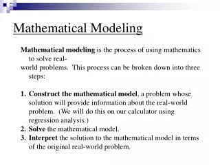
MATHEMATICAL MODELING. Example 5- Aircraft Pitch. Pitch angle: is the angle between the center line of the roll axis of the aircraft (nose to tail,the longitudinal axis) and the horizon. Angle of attack is the angle between the chord line of an airfoil and the relative wind


MATHEMATICAL MODELING
E N D
Presentation Transcript
Example 5- Aircraft Pitch • Pitch angle: is the angle between the centerline of the roll axis of the aircraft (nose to tail,the longitudinal axis) and the horizon. • Angle of attack is the angle between the chord line of an airfoil and the relative wind through which it is moving.
The angle of attack and the pitch angle are usually different in flights. • Sometimes the pitch angle may be positive or negative in normal flight, but the angle of attack is always positive.
There are 4 forces involved with flight: i. Lift ii. Weight iii. Thrust iv. Drag
Axis of flight Three axis’ of flight include: Pitch, Roll, and Yaw 1. Roll is controlled by the air flow across the ailerons 2. Yaw is controlled by the air flow across the rudder 3. Pitch is controlled by the air flow across the elevators.
Design Requirements of Air-craft • Overshoot less than 10% • b) Rise time less than 2 seconds • c) Settling time less than 10 seconds • d) Steady-state error less than 2%
Aircraft Pitch: System Modeling • The of equations governing the motion of an aircraft are a very complicated set of six nonlinear coupled differential equations. • However, under certain assumptions, they can be decoupled and linearized into longitudinal and lateral equations.
Aircraft pitch is governed by the longitudinal dynamics. In this example we will design an autopilot that controls the pitch of an aircraft. • We will assume that the aircraft is in steady-state at constant altitude and velocity.
Thus, the thrust, drag, weight and lift forces balance each other in the x- and y-directions. • We will also assume that a change in pitch angle will not change the speed of the aircraft under any circumstance (unrealistic but simplifies the problem a bit).
Transfer Function • Before finding the transfer function and state-space models, let's plug in some numerical values to simplify the modeling equations shown above: • Above equation become:
To find the transfer function of the above system, we need to take the Laplace transform of the above modeling equations. • The Laplace transform of the above equations are shown below.
Aircraft Pitch: System Analysis System analysis contain: • Open loop response. • Close loop response.
Open loop response: MATLAB (M-FILE CODE)
Conclusions From the above plot, we see that the open-loop response does not satisfy the design criteria at all. In fact, the open-loop response is unstable.
Closed-loop response MATLAB (M-FILE CODE)
Conclusions The above plot again demonstrates that this closed- loop system does not meet the given design requirements.
Example 6: Trajectory Motion with Aerodynamic Drag y axis x axis
Example 6 Solve the following differential equations for cd={0.1, 0.3,0.5} N/m.
Solution • To solve the given two differential equations we have to reduce each of them into two first order differential equations. Let
The above equations reduce to the following first order differential equations.
Computational Model • Type the following code in a separate m-file. • The system derivatives must be written in a separate m-file. • Since the name of the function is ‘airdrag’, save the m-file as ‘airdrag.m’ in the current directory.
Computational Model function yp = airdrag(t,y) m = 10; cd = 0.2; g = 9.81; w = m*g; yp = zeros(4,1);
Computational Model yp(1) = y(2); yp(2) = ((-cd/m)*y(2)*(y(2)^2+y(4)^2)^(0.5)); yp(3) = y(4); yp(4) = ((-w/m)-(cd/m)*y(4)*(y(2)^2+y(4)^2)^(0.5)); • Open a new m-file and type the following code for the main program.
Computational Model • This program calls the function ‘airdrag.m’ in order to solve the differential equations. tspan=[0 5]; y0=[0;100;0;10] [t,y]=ode45('airdrag',tspan,y0); plot(y(:,1),y(:,3)) grid
Computational Model xlabel(‘X-Displacement’) ylabel(‘Y-Displacement’) title(‘X vs Y Displacement’) hold on;
Conclusions It can be seen from the plots that as the coefficient of the aerodynamic drag is increased the maximum value of the displacement in the y direction decreases. The value of the displacement in the x direction, for which the displacement in the y direction is maximum, also decreases.