Download

1 / 30
300 likes | 473 Views
This chapter explores Darcy's Law, developed by Henry Darcy during the 19th century while improving Dijon, France's public waterworks. Faced with the challenge of designing effective sand filters for fountains, Darcy conducted experiments to determine how water flows through different geological materials like sand and clay. His findings, published in 1856, laid the foundation for understanding fluid dynamics in porous media. Key experimental setups and variable impacts, such as pressure, length, and cross-sectional area on flow rate, are also detailed.

E N D
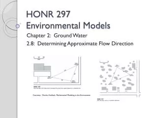
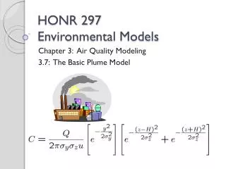
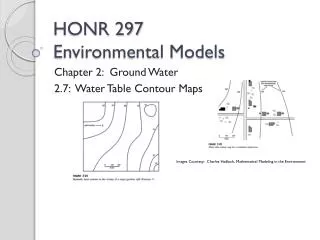
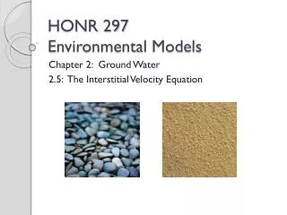
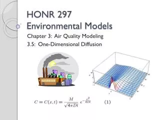
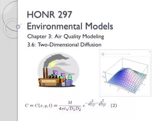
HONR 297Environmental Models Chapter 2: Ground Water 2.4: Darcy’s Law
Henry Darcy (1803 – 1858) • In the mid 19th century, the city of Dijon, France decided to improve and enlarge the city’s public water works. • Henry, Darcy, the the local InspecteurDivisionnaire des Ponts et Chausees (Inspector General of Bridges and Roads), was responsible for this civil engineering program. • One of the challenges faced by Darcy was how to design sand filters for the city’s public fountains. • Henry Darcy Video! Courtesy Wikipedia Commons: http://commons.wikimedia.org/wiki/File:Henry_Darcy.jpg
Henry Darcy • Since there weren’t any models for the flow of fluid through a porous medium, Darcy had to create one. • To do so, he performed his own experiments on the flow of water through sand. • His results, including what we now know as Darcy’s Law, were published in 1856 as an appendix to his 647-page report on the project: Les FontainesPubliques de la Ville de Dijon.
Darcy’s Question • One of the basic questions Darcy wanted to answer was: • How much water could move at what rate through what size filter? ?
Experimental Set-up • The experimental set-up above, based on Figure 2.7 in our text is similar that used by Darcy – all results that follow were observed experimentally by Darcy! • Geologic material (sand, clay, gravel, silt, etc.) is placed in the middle of a tube. • Water in introduced on one end and pushed through the sample material by means of forced a piston. • If water passes through the geologic material easily (sand, gravel, etc.) then minimal force (which means less pressure) needs to be applied. • For material more resistant to flow (clay, silt, etc.), more force (which means greater pressure) has to be applied – sufficient pressure will bring the flow rate back up to what it was for the sand or gravel. Flow Force Water Under Negligible Pressure Water Under Pressure Geologic Sample
Base Set-up for Experiments Length = L • For all experiments that follow, we will use this set-up as a base case. • Assume for each experiment that is performed, the same type of geologic material is placed in the tube. • Suppose for the base set-up, with pressure P, length of material L, and cross-sectional area A, we get a flow rate Q. Flow rate Q Force Cross- Sectional Area is A A Pressure = 0 Pressure = P
Experiment 1 – Double Pressure Length = L • Suppose we increase the force so that the pressure on the left end is doubled to 2P, while all other parameters stay the same. • Question: How will this affect the flow rate on the right end? • Answer: The flow rate will double to 2Q! Flow rate ? More Force Cross- Sectional Area is A A Pressure = 0 Pressure = 2P
Experiment 2 – Double Length Length = 2L • Suppose we use the original amount of force on the left end, but double the sample length to 2L, again leaving all other parameters the same as in the base case. • Question: How will this affect the flow rate on the right end? • Note that the volume of the material resisting the flow has doubled! • Answer: The flow rate will be cut in half to Q/2! Flow rate ? Force Cross- Sectional Area is A Pressure = P A Pressure = 0
Experiment 3 – Double Length and Double Pressure Length = 2L • Now, let’s start with the set-up for the last experiment, but increase the force so that the pressure on the left end is doubled. • Question: How will this affect the flow rate on the right end? • Note that the volume of the material resisting the flow has doubled, but the pressure has increased to compensate for this! • Answer: The flow rate will be the same as the base case – namely Q! Flow rate ? More Force Cross- Sectional Area is A Pressure = 2P A Pressure = 0
Experiment 4 – Double Cross-sectional Area Length = L • Now, let’s suppose that we place two copies of the base-case set-up in parallel. • Question: How much water will be flowing through this new set-up, as compared to the base-case set-up? • Answer: Twice as much water! • Reason: Since we’ve doubled the cross – sectional area of the water pathway through the sample material, this doubles the volume of water that can be pushed through! Cross- Sectional Area is A A Flow Force Pressure = P Pressure = 0 Cross- Sectional Area is A A
Our Observations so Far … • Double Pressure (2P) => Double Flow Rate (2Q) • Double Sample Length (2L) => One Half Flow Rate (Q/2) • Double Cross-Sectional Area (2A) => Double Flow Rate (2Q) • In each case, we were changing a parameter by a factor of two! • What if we changed our parameters by a factor of three? How about K?
Parameter Change Factor • Triple Pressure (3P) => Triple Flow Rate (3Q) • Triple Sample Length (3L) => One Third Flow Rate (Q/3) • Triple Cross-Sectional Area (3A) => Triple Flow Rate (3Q) • K*P => K*Q • K*L => Q/K • K*A => K*Q • So, how is the flow rate related to pressure, length, and cross-sectional area in general?
General Relationships Between Flow Rate and Parameters • The flow rate is proportional to the pressure. • The flow rate is inversely proportional to the sample length. • The flow rate is proportional to the cross-sectional area of the sample. • Mathematically, we can write this as Q = K*P*(1/L)*A (1) where K is a constant of proportionality that will depend on the sample material. • Equation (1) provides an initial mathematical model to describe the flow rate of through the sample material!
A Revised Experimental Set-up! • Instead of using a piston at the left end to control pressure, we can use columns of water to do the same thing (this is what Darcy actually did). • If the left column of water is higher than the right column, then the net pressure will be equal to the difference in water column heights, which we will denote by h, i.e. h = h1 – h2 Flow Flow Height = h1 Height = h2 Flow Geologic Material, length L, cross-section A Reference level for measuring heights, for example, sea level.
A Revised Mathematical Model • Replacing pressure P with change in height h, our flow rate equation (1) becomes Q = K*h*(1/L)*A. • In this expression, Q is the total flow rate through the sample, measured in units that represent volume per unit time, for example gallons per minute, cubic feet per day, etc. Flow Flow Height = h1 Height = h2 Flow Geologic Material, length L, cross-section A Reference level for measuring heights, for example, sea level.
Hydraulic Conductivity • In order for our flow equation (1) to make sense, we need to figure out the units on the constant of proportionality, K, which we will call the hydraulic conductivity. • Units of Q: [Q] = (length^3)/(time) • Units of h: [h] = length • Units of length: [L] = length • Units of area A: [A] = length^2
Hydraulic Conductivity • Units of hydraulic conductivity K: [K] = [(Q*L)/(h*A)] = ((length^3)/(time)*length)/(length*length^2) = length/time • Thus, the units for hydraulic conductivity are [K] = length/time! • Examples of hydraulic conductivity (found experimentally) for various materials are given in our text on page 26 – Table 2.1. • Notice that the hydraulic conductivity of gravel and sand is higher than that for silt or clay – does this make sense with which materials allow water to flow more freely?
Hydraulic Gradient • We need to define one more quantity, after which we can present Darcy’s Law! • This is related to our Experiment 3 above, in which we noted that if we double the sample length and double the pressure, the flow rate stays the same. • The hydraulic gradient, i, is defined by i = h/L. • The hydraulic gradient describes the change in pressure over the change in length of the sample – note that the hydraulic gradient is dimensionless, as [i] = [h/L] = length/length. • Replacing h/L with i in equation (1) yields Darcy’s Law!
Darcy’s Law • Q = K i A • where • Q is the volumetric flow rate • K is the hydraulic conductivity of the geologic material • i is the hydraulic gradient, with i = h/L. • A is the cross-sectional area
Hydraulic Head • Definition: • The height of the water level at any point is called the (hydraulic) head. The change in hydraulic head between two points is called the head loss or change in head and denoted h.
Example 1 • Imagine an underground sand aquifer that is 40 feet thick, 200 feet wide, and has a hydraulic conductivity of 25 ft/day. Two test wells 750 feet apart are drilled into the aquifer, along the axis of flow, and the measured head values at these wells were found to be 120 and 114 feet, respectively. • (a) Draw a really clear diagram of this situation. • (b) Find the total flow rate in a given cross section of the aquifer.
Example 1 • (a) Sketch diagram of situation on board. • (b) Use Darcy’s Law with the following: • Cross-sectional area is A = (40 ft)(200 ft) = = 8000 ft^2. • Change in head is h = h1 – h2 = = 120 ft – 114 ft = 6 ft. • Length is L = 750 ft • Thus, the hydraulic gradient is i = h/L = (6 ft)/(750 ft). • Finally, the hydraulic conductivity is K = 25 ft/day. • Thus, we have from Darcy’s Law: • Q = K i A = K (h/L) A =(25 ft/day)(6 ft)/(750 ft)(8000 ft^2) = 1600 (ft^3)/day
Estimating Contamination Concentration • If we know the rate at which a contaminant is leaking into an aquifer, then we can use calculations like those in Example 1 to estimate the concentration of the contaminant in an aquifer! • For contaminant concentration calculations, we assume that once the contaminant enters the aquifer it moves downstream at the same rate as the ground water. • We also assume that the contaminant “immediately” spreads out and becomes uniformly mixed in the water.
Example 2 • As an example, suppose 3 lb of contaminant is leaking into the aquifer from Example 1 each day (say at the left end). • Then, in the course of one day, 1600 cubic feet of water will pass through an imaginary cross-sectional plane perpendicular to the flow of the groundwater. • Also, three pounds of contaminant will pass through this plane each day! • It follows that the concentration of contaminant in the water is C = (3 lb/day)/(1600 (ft^3)/day) = 3/1600 lb/ft^3 = 0.001875 lb/ft^3.
Unit Conversion • Often, one needs to convert results in terms of given units to another set of units. • An example of why this may be necessary is that data from reports may not always be in the units needed for a calculation or data comparison. • Suppose for instance that we want to know the contaminant concentration from Example 2 in kg/m^3.
Example 3 • Convert 0.001875 lb/ft^3 into kg/m^3. • One solution is to use a unit conversion tool such as this one, found online: http://www.calculatorsoup.com/calculators/conversions/density.php. • We can also convert “by hand”! • Use the facts that 1 kg = 2.20462 lb and 1 in = 2.54 cm.
Example 3 • (0.001875 lb/ft^3) =(0.001875 lb/ft^3)*(1 kg/(2.20462 lb)) *(1 ft/(12 in))^3*(1 in/(2.54 cm))^3 *(100 cm/(1 m))^3 = 0.0300347 kg/m^3
Parts per Million (ppm) • Often, concentration of pollutants in ground water are measured in parts per million, denoted “ppm”. • For ground water contamination, we are dealing with contaminant amounts that are measured in units of mass or weight. • For example, if we have contamination concentration given in the following units: [concentration] = mass/volume, • First convert the volume to mass units, then convert the denominator mass units to one million mass units.
Example 4 • From Example 3, we have a contaminant concentration of 0.0300347 kg/m^3. • Use the fact that one cubic meter of water has a mass of 1000 kg to convert this concentration measurement to ppm. • Solution: 0.0300347 kg/m^3 = (0.0300347 kg contaminant)/(m^3 water) *(1 m^3 water)/(1000 kg water) *(10^6 kg water)/(1 million kg water) = (30.0347 kg contaminant)/1million kg water) = 30.0347 ppm
Resources • http://commons.wikimedia.org/wiki/File:Henry_Darcy.jpg • http://www.youtube.com/watch?v=yiTy21mJNM0 • Groetsch, Charles W., Inverse Problems, Mathematical Association of America, 1999. • http://www.calculatorsoup.com/calculators/conversions/density.php