Download
1 / 45
460 likes | 681 Views
Environmental Fate Models. LEVEL I. Merits To assess multi-media environmental concentrations under more realistic conditions To assess a chemicals’ persistence To assess dominant processes To screen substances for the purpose of ranking. Steady-State & Equilibrium. Cwater. GILL UPTAKE.

E N D
Merits To assess multi-media environmental concentrations under more realistic conditions To assess a chemicals’ persistence To assess dominant processes To screen substances for the purpose of ranking
Steady-State & Equilibrium Cwater GILL UPTAKE GILL ELIMINATION
Steady-State Flux Equation: “Mass Balance Equation” dMF/dt = DWF.fW - DFW.fF = 0 DWF.fW = DFW.fF fF/fW = DWF/DFW = 1.0 CF/CW = fF.ZF/fW.ZW = ZF/ZW = KFW Equilibrium
Steady-State Flux Equation: “Mass Balance Equation” d(CF.VF)/dt = kWF.VF.CW - kFW.VF.CF = 0 dCF/dt = kWF.CW - kFW.CF = 0 kWF.CW = kFW.CF CF/CW = kWF/kFW = KFW Equilibrium
Steady-State & Equilibrium Cwater GILL UPTAKE METABOLISM GILL ELIMINATION
Steady-State Flux Equation: “Mass Balance Equation” dMF/dt = DWF.fW - DFW.fF - DM.fF = 0 DWF.fW = DFW.fF +DM.fF fF/fW = DWF/(DFW +DM) < 1.0 CF/CW = (ZF/ZW). DWF/(DFW +DM)< KFW Steady-State
Steady-State Flux Equation: “Mass Balance Equation” dCF/dt = kWF.CW - kFW.CF - kM.CF = 0 kWF.CW = kFW.CF +kM.CF CF/CW = kWF/(kFW +kM) < 1.0 CF/CW = kWF/(kFW +kM)< KFW Steady-State
What is the difference between Equilibrium & Steady-State?
Question : What is the concentration of chemical X in the water (fish kills?) Tool : Use steady-state mass-balance model Volatilisation Emission Outflow CW=? Reaction Sedimentation Lake
Concentration Format dMW/dt = E - kV.MW - kS.MW - kO.MW - kR.MW dMW/dt = E - (kV + kS+ kO+ kR).MW 0 = E - (kV + kS+ kO+ kR).MW E = (kV + kS+ kO+ kR).MW MW = E/(kV + kS+ kO+ kR) & CW = MW/VW
Fugacity Format d(VW ZW.fW )/dt = E - DV.fW - DS.fW - DO.fW - DR.fW dfW/dt = E - (DV + DS+ DO+ DR).fW 0 = E - (DV + DS+ DO+ DR).fW E = (DV + DS+ DO+ DR).fW fW = E/ (DV + DS+ DO+ DR) & CW = fW.ZW
Steady-state mass-balance model: 2 Media Volatilisation Emission Outflow Settling CW=? Reaction Resuspension CS=? Burial
Water: dMw/dt = Input + ksw.Ms - kw.Mw - kws.Mw = 0 Sediments: dMs/dt = kws.Mw - kb.Ms - ksw.Ms = 0
From : Eq. 2 kws.Mw = kb.Ms + ksw.Ms Ms = kws.Mw / (kb + ksw) Substitute in eq. 1 Input + ksw.{kws.Mw / (kb + ksw)} = kw.Mw + kws.Mw Input = kw.Mw + kws.Mw - ksw.{kws.Mw / (kb + ksw)}
In Fugacity Format Water: dMw/dt = Input + Dsw.fs - Dw.fw - Dws.fw = 0 Sediments: dMs/dt = Dws.fw - Db.fs - Dsw.fs = 0
From : Eq. 2 Dws.fw = Db.fs + Dsw.fs fs = Dws.fw / (Db + Dsw) Substitute in eq. 1 Input + Dsw.{Dws.fw / (Db + Dsw)} = Dw.fw + Dws.fw Input = Dw.fw + Dws.fw - Dsw.{Dws.fw / (Db + Dsw)}
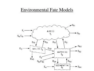
Level III fugacity Model: Steady-state in each compartment of the environment Flux in = Flux out Ei + Sum(Gi.CBi) + Sum(Dji.fj)= Sum(DRi + DAi + Dij.)fi For each compartment, there is one equation & one unknown. This set of equations can be solved by substitution and elimination, but this is quite a chore. Use Computer
Level II fugacity Model: Steady-state over the ENTIRE environment Flux in = Flux out E + GA.CBA + GW.CBW = GA.CA + GW.CW All Inputs = GA.CA + GW.CW All Inputs = GA.fA .ZA + GW.fW .ZW Assume equilibrium between media : fA= fW All Inputs = (GA.ZA + GW.ZW).f f = All Inputs / (GA.ZA + GW.ZW) f = All Inputs / Sum (all D values)
Reaction Rate Constant for Environment: Fraction of Mass of Chemical reacting per unit of time kR = Sum(Mi.ki) / Mtotal tREACTION = 1/kR
Removal Rate Constant for Environment: Fraction of Mass of Chemical removed per unit of time by advection kA = Sum(Gi.Ci) / Mtotal tADVECTION = 1/kA
Total Residence Time in Environment: ktotal = kA + kR = E/M tRESIDENCE = 1/kTOTAL = 1/kA +1/kR 1/tRESIDENCE = 1/tADVECTION +1/tREACTION
Application of the Models • To assess concentrations in the environment • (if selecting appropriate environmental conditions) • To assess chemical persistence in the environment • To determine an environmental distribution profile • To assess changes in concentrations over time.
Fugacity Models Level 1 : Equilibrium Level 2 : Equilibrium between compartments & Steady-state over entire environment Level 3 : Steady-State between compartments Level 4 : No steady-state or equilibrium / time dependent
Recipe for developing mass balance equations 1. Identify # of compartments 2. Identify relevant transport and transformation processes 3. It helps to make a conceptual diagram with arrows representing the relevant transport and transformation processes 4. Set up the differential equation for each compartment 5. Solve the differential equation(s) by assuming steady-state, i.e. Net flux is 0, dC/dt or df/dt is 0.