Download
1 / 15
150 likes | 347 Views
HONR 297 Environmental Models. Chapter 2: Ground Water 2.8: Determining Approximate Flow Direction. Courtesy: Charles Hadlock , Mathematical Modeling in the Environment. Key Factors for Flow Direction.

E N D
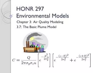
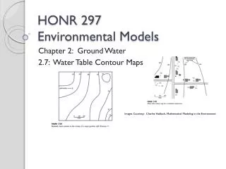
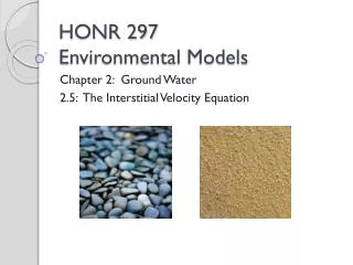
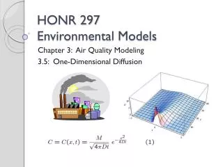
HONR 297Environmental Models Chapter 2: Ground Water 2.8: Determining Approximate Flow Direction Courtesy: Charles Hadlock, Mathematical Modeling in the Environment
Key Factors for Flow Direction • From the last section, we saw that the keys to determining flow direction of ground water were hydraulic gradient i = Δh/L and hydraulic contour lines from a given water table contour map. • Using these ideas along with the Key Idea that ground water flows perpendicular to hydraulic head contour lines, we were able to find flow direction and travel time! Courtesy: Charles Hadlock, Mathematical Modeling in the Environment
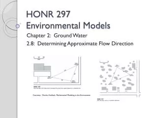
Determining Flow Directions from Field Data • Suppose we are given the scenario illustrated in Figure 2.29 of our text, shown to the right. • In this case, there is a commercial building with three wells drilled into the ground to the east of the building. • Can you guess how one can determine the flow direction of ground water flow from this data? Courtesy: Charles Hadlock, Mathematical Modeling in the Environment
Determining Flow Directions from Field Data Courtesy: Charles Hadlock, Mathematical Modeling in the Environment
Determining Flow Directions from Field Data – Intermediate Well • Identify the well head that has a value between the other two. • In this case, Well 1’s head level of 37 feet is between Well 3’s head level (34 feet) and Well 2’s head level (40 feet). Courtesy: Charles Hadlock, Mathematical Modeling in the Environment
Determining Flow Directions from Field Data – Intermediate Point • Since the hydraulic head at Well 1 is between the hydraulic heads of Well 3 and Well 2, there must also be some point along the line segment from Well 3 to Well 2 at which the head value is the same as that for Well 1. • The reason for this is that the hydraulic head must change from Well 3 to Well 2 in a continuous fashion – thus it must hit 37 feet somewhere between these two wells! (Think of contour lines passing through each well …) Courtesy: Charles Hadlock, Mathematical Modeling in the Environment
Determining Flow Directions from Field Data – Intermediate Point • Find the location of this intermediate point P between Wells 3 and 2 – to do so, we can use the idea of proportions! • Since the change in head level from Well 3 to Well 1, relative to the change in head level from Well 3 to Well 2 is (37-34)/(40-34) = 3/6 = 1/2, most likely the distance from Well 3 to the intermediate point P relative to the distance from Well 3 to Well 2 should be the same, i.e. (Distance from Well 3 to point P)/(Distance from Well 3 to Well 2) = 1/2. P Courtesy: Charles Hadlock, Mathematical Modeling in the Environment
Determining Flow Directions from Field Data – Intermediate Point • It follows that Distance from Well 3 to point P = (1/2)(Distance from Well 3 to Well 2) = (1/2)(350 feet) = 175 feet. P Courtesy: Charles Hadlock, Mathematical Modeling in the Environment
Determining Flow Directions from Field Data – Contour Line • Next, we construct our best estimate of the contour line with height 37 feet. • We have two points that are on the 37 – foot contour line, Well 1 and point P. • Since we don’t know any more about the contour line that contains these points, it is standard practice to draw a straight line through these points! P Courtesy: Charles Hadlock, Mathematical Modeling in the Environment
Determining Flow Directions from Field Data – Flow Direction • After we’ve drawn the contour line, we can estimate the groundwater flow direction. • Using the Key Idea, choose a point Q on the 37 – foot contour line so that a perpendicular line segment from Q passes through Well 3 (as shown in Figure 2.30)! Courtesy: Charles Hadlock, Mathematical Modeling in the Environment
Determining Flow Directions from Field Data – Flow Direction Courtesy: Charles Hadlock, Mathematical Modeling in the Environment
Determining Hydraulic Gradient from Field Data • Finally, we can calculate the hydraulic gradient i in the direction of flow! • Using the head levels at point Q and Well 3, we can compute Δh. • The distance L between point Q and Well 3 can be measured off of the map, using the given scale! • We find that i = Δh/L = (37 ft – 34 ft)/(150 ft) = 3/150 = 0.02 Courtesy: Charles Hadlock, Mathematical Modeling in the Environment
Additional Example • Consider the situation shown to the right (Figure 2.31 in Hadlock), which is analogous to the example treated above. Determine the general direction of flow and the corresponding hydraulic gradient.
Additional Example Courtesy: Charles Hadlock, Mathematical Modeling in the Environment
Resources • Charles Hadlock, Mathematical Modeling in the Environment, Section 2.8 • Figures 2.29, 2.30, and 2.31 used with permission from the publisher (MAA).