Sampling distributions for sample means
Sampling distributions for sample means. IPS chapter 5.2. © 2006 W.H. Freeman and Company. Objectives (IPS chapter 5.2). Sampling distribution of a sample mean Sampling distribution of x bar For normally distributed populations The central limit theorem Weibull distributions.

Sampling distributions for sample means
E N D
Presentation Transcript
Sampling distributions for sample means IPS chapter 5.2 © 2006 W.H. Freeman and Company
Objectives (IPS chapter 5.2) Sampling distribution of a sample mean • Sampling distribution of x bar • For normally distributed populations • The central limit theorem • Weibull distributions
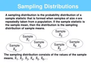
Reminder: What is a sampling distribution? The sampling distribution of a statistic is the distribution of all possible values taken by the statistic when all possible samples of a fixed size n are taken from the population. It is a theoretical idea — we do not actually build it. The sampling distribution of a statistic is the probability distribution of that statistic.
Sampling distribution of x bar We take many random samples of a given size n from a population with mean mand standard deviations. Some sample means will be above the population mean m and some will be below, making up the sampling distribution. Sampling distribution of “x bar” Histogram of some sample averages
For any population with mean m and standard deviation s: • The mean, or center of the sampling distribution of x bar, is equal to the population mean m :mx = m. • The standard deviation of the sampling distribution is s/√n, where n is the sample size :sx= s/√n. Sampling distribution of x bar s/√n m
Mean of a sampling distribution of x bar: There is no tendency for a sample mean to fall systematically above or below m, even if the distribution of the raw data is skewed. Thus, the mean of the sampling distribution of x bar is an unbiasedestimate of the population mean m— it will be “correct on average” in many samples. • Standard deviation of a sampling distribution of x bar: The standard deviation of the sampling distribution measures how much the sample statistic x bar varies from sample to sample. It is smaller than the standard deviation of the population by a factor of √n. Averages are less variable than individual observations.
For normally distributed populations When a variable in a population is normally distributed, the sampling distribution of x bar for all possible samples of size n is also normally distributed. Sampling distribution If the population is N(m, s) then the sample means distribution is N(m, s/√n). Population
IQ scores: population vs. sample In a large population of adults, the mean IQ is 112 with standard deviation 20. Suppose 200 adults are randomly selected for a market research campaign. • The distribution of the sample mean IQ is: A) Exactly normal, mean 112, standard deviation 20 B) Approximately normal, mean 112, standard deviation 20 C) Approximately normal, mean 112 , standard deviation 1.414 D) Approximately normal, mean 112, standard deviation 0.1 C) Approximately normal, mean 112 , standard deviation 1.414 Population distribution : N(m = 112; s= 20) Sampling distribution for n = 200 is N(m = 112; s /√n = 1.414)
z = −1.5, P(z < −1.5) = 0.0668 ≈ 7% If instead measurements are taken on 4 separate days, what is the probability of such a misdiagnosis? Application Hypokalemia is diagnosed when blood potassium levels are low, below 3.5mEq/dl. Let’s assume that we know a patient whose measured potassium levels vary daily according to a normal distribution N(m = 3.8, s = 0.2). If only one measurement is made, what is the probability that this patient will be misdiagnosed hypokalemic? z = −3, P(z < −1.5) = 0.0013 ≈ 0.1% Note: Make sure to standardize (z) using the standard deviation for the sampling distribution.
Practical note • Large samples are not always attainable. • Sometimes the cost, difficulty, or preciousness of what is studied drastically limits any possible sample size. • Blood samples/biopsies: No more than a handful of repetitions acceptable. Often, we even make do with just one. • Opinion polls have a limited sample size due to time and cost of operation. During election times, though, sample sizes are increased for better accuracy. • Not all variables are normally distributed. • Income, for example, is typically strongly skewed. • Is still a good estimator of m then?
The central limit theorem Central Limit Theorem: When randomly sampling from any population with mean mand standard deviation s, when n is large enough, the sampling distribution of x bar is approximately normal: ~N(m, s/√n). Population with strongly skewed distribution Sampling distribution of for n = 2 observations Sampling distribution of for n = 10 observations Sampling distribution of for n = 25 observations
Income distribution Let’s consider the very large database of individual incomes from the Bureau of Labor Statistics as our population. It is strongly right skewed. • We take 1000 SRSs of 100 incomes, calculate the sample mean for each, and make a histogram of these 1000 means. • We also take 1000 SRSs of 25 incomes, calculate the sample mean for each, and make a histogram of these 1000 means. Which histogram corresponds to the samples of size 100? 25? $$$
How large a sample size? It depends on the population distribution. More observations are required if the population distribution is far from normal. • A sample size of 25 is generally enough to obtain a normal sampling distribution from a strong skewness or even mild outliers. • A sample size of 40 will typically be good enough to overcome extreme skewness and outliers. In many cases, n = 25 isn’t a huge sample. Thus, even for strange population distributions we can assume a normal sampling distribution of the mean and work with it to solve problems.
Sampling distributions Atlantic acorn sizes (in cm3) — sample of 28 acorns: • Describe the histogram. What do you assume for the population distribution? • What would be the shape of the sampling distribution of the mean: • For samples of size 5? • For samples of size 15? • For samples of size 50?
Further properties Any linear combination of independent random variables is also normally distributed. More generally, the central limit theorem is valid as long as we are sampling many small random events, even if the events have different distributions (as long as no one random event dominates the others). Why is this cool? It explains why the normal distribution is so common. Example: Height seems to be determined by a large number of genetic and environmental factors, like nutrition. The “individuals” are genes and environmental factors. Your height is a mean.
Weibull distributions There are many probability distributions beyond the binomial and normal distributions used to model data in various circumstances. Weibull distributions are used to model time to failure/product lifetime and are common in engineering to study product reliability. Product lifetimes can be measured in units of time, distances, or number of cycles for example. Some applications include: • Quality control (breaking strength of products and parts, food shelf life) • Maintenance planning (scheduled car revision, airplane maintenance) • Cost analysis and control (number of returns under warranty, delivery time) • Research (materials properties, microbial resistance to treatment)
Density curves of three members of the Weibull family describing a different type of product time to failure in manufacturing: Infant mortality: Many products fail immediately and the remainder last a long time. Manufacturers only ship the products after inspection. Early failure: Products usually fail shortly after they are sold. The design or production must be fixed. Old-age wear out: Most products wear out over time and many fail at about the same age. This should be disclosed to customers.