Ch 7 - Sampling Distribution
Ch 7 - Sampling Distribution. Tuesday, January 3, 3012. The Airport Problem. This activity will review binomial calculations and introduce the idea of sampling distribution of sample proportions using simulation You will need your TI-83/84 calculators.

Ch 7 - Sampling Distribution
E N D
Presentation Transcript
Ch 7 - Sampling Distribution • Tuesday, January 3, 3012
The Airport Problem • This activity will review binomial calculations and introduce the idea of sampling distribution of sample proportions using simulation • You will need your TI-83/84 calculators
At Guadalajara Airport in Mexico, passengers must claim their luggage and then proceed to Customs. In the Customs area, each passenger will press a button that activates a modified stoplight. This light has only red and green bulbs. If the green lights shows, the passenger is free to go. If the light turns red, then Customs agents will inspect the passenger’s luggage. Customs officials claim that the light has a probability of 0.30 of showing red on any press of the button.
You have 20 minutes to start the activity that I am passing out. It is due at the beginning of class tomorrow. You do not have to draw the graphs, if you are describing them. Remember your “SOCS!” You can look at them on your calculators.
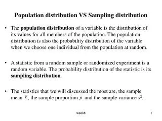
Vocabulary • Population (review) • Sample (review) • Parameter • Statistic • *Hint: the p’s and the s’s go together!
Notation • notation is very important, and you will loose points on the exam if you use the wrong notation (as well as if you use the wrong word) • Population mean: • Sample mean: x • Population Proportion: p • Sample Proportion: p _ ^
7.1 - Continued • Each of you will randomly select 5 cards from a shuffled deck and note the median value. Then replace your cards. • You will do this 2 times each • After you are finished, record the value of the sample median on the dotplot on the board. Use a lower case “m” instead of a dot since we are talking about a sample and not a population. • Then we will describe what we see: Shape, Center (mean), Spread (standard deviation), and Outliers! Wednesday, January 4, 2012
Sampling Distribution The sampling distribution of a statistic is the distribution of values taken by the statistic in all possible samples of the same size from a population. For example, in our card activity if we were able to take every possible sample of size 5 and record the outcomes, that would be the sampling distribution of the median of cards 2 through 10 when selecting 5 cards. That would be 36 nCr 5 = 376,992 different samples! It’s very time consuming to take all possible samples, instead simulations are done to imitate the process we just did. (FATHOM)
Using Fathom to simulate choosing 500 SRSs of size 5 from the deck of cards 2 though 10 and finding the sample medians produced the following dotplot.
Distribution, Distribution, Distribution... • There are 3 different types of distributions: • 1. Population Distribution • 2. Distributions of Sample Data • 3. Sampling Distributions • *Yes, there is a difference between sample distribution and sampling distribution
What’s the difference between the 3 distributions? • A population distribution is one graph of everything possible as a whole. • For our card activity, we would have a bar graph with 9 bars (2 - 10) with a frequency of 4 each. A distribution of sample data is an individual graph depicting each outcome from the sample you drew from the population. For our card activity, we would have a separate bar graph for each sample you drew showing all the cards you drew and their frequencies. Sampling distribution describes how a statistic varies in many, many samples of the population. You are no longer looking at the individual elements in the sample/population. For our card activity, it would have been the simulation we ran on fathom showing the different values of the medians of our samples.
Why didn’t we find the standard deviation since we estimated the mean for the center? Describing Sampling Distributions Let’s describe the dotplot of the simulation of 500 SRSs of size 5 from our deck of cards: Shape: Center: Spread: Outliers: roughly symmetric with a single peak at 6 the mean of the sample medians is about 6 most of the values fall between 4 and 8 with a few at 2 and 10 there doesn’t appear to be any outliers
More questions about our card simulation: • Was that a sampling distribution? • If someone claims to set up the same activity and they select a sample of size 5 and get a median of 4, is that convincing evidence that they set their deck up wrong?
Biased and Unbiased Estimators • This is different than the sampling process being biased. When using an estimator (i.e. a measure of center or spread) we are assuming the sampling process is not biased. • The actual statistic we are finding can be biased or unbiased as well.
Biased or Unbiased? So which sample statistics are biased and which are unbiased? To find out, let’s collect some quantitative data: 1. On the piece of paper given to you write how many hours of sleep you got last night. 2. Each of you will randomly select a sample of 4 cards. 3. You will need to record the following information: the person’s initials, the hours of sleep they got, the sample mean, and the sample range. 4. Replace the cards, shake the bag, and draw another sample of size 4 and record the same information. 5. Pass the bag to the next person then record your sample mean and sample range on the corresponding dotplots on the board. 6. Once everyone plots their data, we will analyze it and compare it to the population mean and population range.
7.2 - Sample Proportions • Remember your notation: • population parameter is p • sample proportion is p ^ Thursday, January 5, 2012
Penny Activity • Let’s look at the population dotplot. Describe what you see.
Penny for you thoughts • Take a sample of size 5 from the population • Calculate p = the proportion of pennies minted in the 2000s • Replace the pennies and repeat a second and third time. • Record your values on the dotplot on the board with p instead of dots. ^ ^
Penny for you thoughts • Take a sample of size 10 from the population • Calculate p = the proportion of pennies minted in the 2000s • Replace the pennies and repeat a second and third time. • Record your values on the dotplot on the board with p instead of dots. ^ ^
Penny for you thoughts • Take a sample of size 20 from the population • Calculate p = the proportion of pennies minted in the 2000s • Replace the pennies and repeat a second and third time. • Record your values on the dotplot on the board with p instead of dots. ^ ^
Compare the 4 graphs Shapes? Centers? Spreads?
More Notations • We have a population, we take a sample, and find some proportion. • If we want to investigate those sample proportions we can find the mean and standard deviation of the sampling distribution of the sample proportions. • mean of sample proportions: • standard deviation of sample proportions: ^ ^
Sampling Distribution of p ^ • SHAPE: sometimes it can be approximated by the Normal curve. It depends on the sample size n and the population proportion p. • CENTER: = p because p is an unbiased estimator of p. • SPREAD: gets smaller as n gets larger. The value of depends on both n and p. ^ ^ ^ ^ p. 436 shows a good, small proof of why these are true
Sampling Distribution of a Sample Proportion • Choose an SRS of size n from a population of size N with proportion p of successes. Let p be the sample proportion of successes. Then: • the mean of the sampling distribution of p is = p • the standard deviation of the sampling distribution of p is • AS LONG AS THE 10% CONDITION IS SATISFIED: • if and , the Normal conditions are satisfied and the sampling distribution of p is approximately Normal. ^ ^ ^ ^ ^ ^ Formulas are on your formula sheet
The superintendent of a large school district wants to know what proportion of middle school students in her district are planning on attending a four-year college or university. Suppose that 80% of all middle school students in her district are planning on attending a four-year college or university. What is the probability that an SRS of size 125 will give a result within 7 percentage points of the true value? • We will use the 4-step method to solve this problem.
State • We want to find the probability that the percentage of middle school students that plan to attend a 4-year college or university falls between 73% and 75% • or in symbols: P(0.73 p 0.78) ^
Plan ^ • = 0.80. • Since the school district is large, we’ll assume the 10% condition is satisfied and there are more than 1250 students. (10*125 = 1250). So, = 0.036 ^ We can consider the distribution of p to be approximately Normal since the following are true: np = 125(.8) = 100 > 10 = 125(.2) = 25 > 10
Do ^ • P(0.73 0.87) = normalcdf(0.73, 0.87, 0.80, 0.036) = 0.948 • If you want full credit on the exam, you must have clearly said everything in the “Plan” step and these calculations will receive full credit. Sketching a Normal curve will help. You can also use Table A to find the answer. Remember to standardize (z-score) first!
Conclude • About 95% of all SRSs of size 125 will give a sample proportion within 7 percentage points of the true proportion of middle school students who want to attend a four-year college or university.
7.3 - Sample Means Friday, January 6, 2012
Back to our pennies! • This activity is very similar to our first activity. In the first one we compared the population proportion of pennies minted in the 2000s to the sample proportion of pennies minted in the 2000s. • This time we will look at the sample distribution of the sample means of the year the pennies were minted
1st: take an SRS of 5 pennies from the population and record their years. • 2nd: replace your sample then repeat two more times. • 3rd: find the mean year for each of your 3 samples. These are your sample means, x • 4th: record your sample means on the appropriate dotplot. Use x’s instead of dots. _ _ After everyone has done this, repeat this process again with SRSs of size 10 and size 25.
Compare the 4 graphs Shapes? Centers? Spreads?
More Notation! • Mean of the sampling distribution: • Standard deviation of the sampling distribution of the sample means: • All of the notations in this chapter are very important and very similar. You will loose credit for using the wrong notations on the exam. So if you can’t remember it’s always best to write out what you are finding rather than try to use a notation. _ _
Suppose that x-bar is the mean of an SRS of size n drawn from a large population with mean and standard deviation , it does not matter what shape the population has. The mean of the sampling distribution of x is The standard deviation of the sampling distribution of x is as long as the 10% condition is satisfied! _ _ _ _ These formulas are on your formula sheet
_ _ • If you are asked to find the sampling distribution of x, these means to state if it is Normal and find the mean and standard deviation. • Hint: if the population itself is approximately Normal, then so is the sampling distribution of x. • Hint: Please read carefully! Make sure you know if you are using the population standard deviation or the sample means standard deviation before you standardize or use your normalcdf on your calculator.
A grinding machine in an auto parts plant prepares axels with a target diameter mu = 40.125 mm. The machine has some variability, so the standard deviation of the diameters is sigma = 0.002 mm. The machine operator inspects a random sample of 4 axles each hour for quality control purposes and records the sample mean diameter x. _ a) Assuming the process is working properly, what are the mean and standard deviation of the sampling distribution of x? - _ b) Can you find the probability that x is within .05 mm if you are choosing an SRS of 100 axels? Explain c) In order for you to pass this inspection the standard deviation of the sampling distribution of x needs to be 0.0005 mm. How many axels would you have to sample?
The composite scores of individual students on the ACT in 2009 followed a Normal distribution with mean 21.1 and standard deviation 5.1. • a) What is the probability that a single student randomly chosen form all those taking the test scores 23 or higher? Show your work. • b) Now take an SRS of 50 students who took the test. What is the probability that the mean score x of these students is 23 or higher?
What if the population shape is not Normal? http://onlinestatbook.com/stat_sim/sampling_dist/index.html Monday, January 9, 2012
Central Limit Theorem • Draw an SRS of size n from any population with mean and finite standard deviation • CLT - when n is large, the sampling distribution of the sample means x is approximately Normal. _ NOTE: this is of the sample means, not just any sample!!!
How large is large? • In order for the Normal conditions to apply for the sample means, and the population is not Normal the CLT will apply in most cases if
The number of flaws per square yard in a type of carpet material varies with the mean 1.6 flaws per square yard and standard deviation 1.2 flaws per square yard. The population distribution cannot be Normal, because a count takes only whole-number values. An inspector studies 200 square yards of material, records the number of flaws found in each square yard, and calculates x, the mean number of flaws per square yard inspected. Find the probability that the mean number of flaws exceeds 2 per square yard. _
State • What’s the probability that the mean number of flaws per square yard of carpet is more than 2?
Plan • The mean of the sampling distribution of the sample means is • 10% condition is met since there’s more than 2000 square yards of carpet, so • Since the sample size is large, 200 > 30, we can safely use the Normal distribution as an approximation for the sampling distribution of x _ _ _
Do • P(x > 2) = normalcdf(2, 100, 1.6, 0.085) = 0
Conclude • There is virtually no chance that the average number of flaws per yard in the sample will be greater than 2.