Run-time Environments
390 likes | 407 Views
This lecture covers the management of run-time resources, the correspondence between static and dynamic structures, and storage organization for code generation.

Run-time Environments
E N D
Presentation Transcript
Run-time Environments Lecture 8 Prof. Necula CS 164 Lecture 14
Status • We have covered the front-end phases • Lexical analysis • Parsing • Semantic analysis • Next are the back-end phases • Optimization • Code generation • We’ll do code generation first . . . Prof. Necula CS 164 Lecture 14
Run-time environments • Before discussing code generation, we need to understand what we are trying to generate • There are a number of standard techniques for structuring executable code that are widely used Prof. Necula CS 164 Lecture 14
Outline • Management of run-time resources • Correspondence between static (compile-time) and dynamic (run-time) structures • Storage organization Prof. Necula CS 164 Lecture 14
Run-time Resources • Execution of a program is initially under the control of the operating system • When a program is invoked: • The OS allocates space for the program • The code is loaded into part of the space • The OS jumps to the entry point (i.e., “main”) Prof. Necula CS 164 Lecture 14
Low Address Code Memory High Address Memory Layout Other Space Prof. Necula CS 164 Lecture 14
Notes • Our pictures of machine organization have: • Low address at the top • High address at the bottom • Lines delimiting areas for different kinds of data • These pictures are simplifications • E.g., not all memory need be contiguous • In some textbooks lower addresses are at bottom Prof. Necula CS 164 Lecture 14
What is Other Space? • Holds all data for the program • Other Space = Data Space • Compiler is responsible for: • Generating code • Orchestrating use of the data area Prof. Necula CS 164 Lecture 14
Code Generation Goals • Two goals: • Correctness • Speed • Most complications in code generation come from trying to be fast as well as correct Prof. Necula CS 164 Lecture 14
Assumptions about Execution • Execution is sequential; control moves from one point in a program to another in a well-defined order • When a procedure is called, control eventually returns to the point immediately after the call Do these assumptions always hold? Prof. Necula CS 164 Lecture 14
Activations • An invocation of procedure P is an activationof P • The lifetime of an activation of P is • All the steps to execute P • Including all the steps in procedures that P calls Prof. Necula CS 164 Lecture 14
Lifetimes of Variables • The lifetimeof a variable x is the portion of execution in which x is defined • Note that • Lifetime is a dynamic (run-time) concept • Scope is a static concept Prof. Necula CS 164 Lecture 14
Activation Trees • Assumption (2) requires that when P calls Q, then Q returns before P does • Lifetimes of procedure activations are properly nested • Activation lifetimes can be depicted as a tree Prof. Necula CS 164 Lecture 14
g f g Example Class Main { g() : Int { 1 }; f(): Int { g() }; main(): Int {{ g(); f(); }}; } Main Prof. Necula CS 164 Lecture 14
Example 2 Class Main { g() : Int { 1 }; f(x:Int): Int { if x = 0 then g() else f(x - 1) fi}; main(): Int {{f(3); }}; } What is the activation tree for this example? Prof. Necula CS 164 Lecture 14
Example Class Main { g() : Int { 1 }; f(): Int { g() }; main(): Int {{ g(); f(); }}; } Main Stack Main Prof. Necula CS 164 Lecture 14
g Example Class Main { g() : Int { 1 }; f(): Int { g() }; main(): Int {{ g(); f(); }}; } Main Stack Main g Prof. Necula CS 164 Lecture 14
g f Example Class Main { g() : Int { 1 }; f(): Int { g() }; main(): Int {{ g(); f(); }}; } Main Stack Main f Prof. Necula CS 164 Lecture 14
g f g Example Class Main { g() : Int { 1 }; f(): Int { g() }; main(): Int {{ g(); f(); }}; } Main Stack Main f g Prof. Necula CS 164 Lecture 14
Notes • The activation tree depends on run-time behavior • The activation tree may be different for every program input • Since activations are properly nested, a stack can track currently active procedures Prof. Necula CS 164 Lecture 14
Low Address Code Memory Stack High Address Revised Memory Layout Prof. Necula CS 164 Lecture 14
Activation Records • On many machines the stack starts at high-addresses and grows towards lower addresses • The information needed to manage one procedure activation is called an activation record (AR) or frame • If procedure F calls G, then G’s activation record contains a mix of info about F and G. Prof. Necula CS 164 Lecture 14
What is in G’s AR when F calls G? • F is “suspended” until G completes, at which point F resumes. G’s AR contains information needed to resume execution of F. • G’s AR may also contain: • Actual parameters to G (supplied by F) • G’s return value (needed by F) • Space for G’s local variables Prof. Necula CS 164 Lecture 14
The Contents of a Typical AR for G • Space for G’s return value • Actual parameters • Pointer to the previous activation record • The control linkpoints to AR of caller of G • Machine status prior to calling G • Contents of registers & program counter • Local variables • Other temporary values Prof. Necula CS 164 Lecture 14
Example 2, Revisited Class Main { g() : Int { 1 }; f(x:Int):Int {if x=0 then g() else f(x - 1)(**)fi}; main(): Int {{f(3); (*) }};} AR for f: Prof. Necula CS 164 Lecture 14
main Stack After Two Calls to f (**) f 2 result (*) Stack f 3 result Prof. Necula CS 164 Lecture 14
Notes • main has no argument or local variables and its result is never used; its AR is uninteresting • (*) and (**) are return addresses of the invocations of f • The return address is where execution resumes after a procedure call finishes • This is only one of many possible AR designs • Would also work for C, Pascal, FORTRAN, etc. Prof. Necula CS 164 Lecture 14
The Main Point The compiler must determine, at compile-time, the layout of activation records and generate code that correctly accesses locations in the activation record Thus, the AR layout and the code generator must be designed together! Prof. Necula CS 164 Lecture 14
Discussion • The advantage of placing the return value 1st in a frame is that the caller can find it at a fixed offset from its own frame • There is nothing magic about this organization • Can rearrange order of frame elements • Can divide caller/callee responsibilities differently • An organization is better if it improves execution speed or simplifies code generation Prof. Necula CS 164 Lecture 14
Discussion (Cont.) • Real compilers hold as much of the frame as possible in registers • Especially the method result and arguments Prof. Necula CS 164 Lecture 14
Globals • All references to a global variable point to the same object • Can’t store a global in an activation record • Globals are assigned a fixed address once • Variables with fixed address are “statically allocated” • Depending on the language, there may be other statically allocated values Prof. Necula CS 164 Lecture 14
Low Address Code Memory Static Data Stack High Address Memory Layout with Static Data Prof. Necula CS 164 Lecture 14
Heap Storage • A value that outlives the procedure that creates it cannot be kept in the AR method foo() { new Bar } The Bar value must survive deallocation of foo’s AR • Languages with dynamically allocated data use a heap to store dynamic data Prof. Necula CS 164 Lecture 14
Notes • The code area contains object code • For most languages, fixed size and read only • The static area contains data (not code) with fixed addresses (e.g., global data) • Fixed size, may be readable or writable • The stack contains an AR for each currently active procedure • Each AR usually fixed size, contains locals • Heap contains all other data • In C, heap is managed by malloc and free Prof. Necula CS 164 Lecture 14
Notes (Cont.) • Both the heap and the stack grow • Must take care that they don’t grow into each other • Solution: start heap and stack at opposite ends of memory and let the grow towards each other Prof. Necula CS 164 Lecture 14
Low Address Code Memory Static Data Heap High Address Stack Memory Layout with Heap Prof. Necula CS 164 Lecture 14
Data Layout • Low-level details of machine architecture are important in laying out data for correct code and maximum performance • Chief among these concerns is alignment Prof. Necula CS 164 Lecture 14
Alignment • Most modern machines are (still) 32 bit • 8 bits in a byte • 4 bytes in a word • Machines are either byte or word addressable • Data is word aligned if it begins at a word boundary • Most machines have some alignment restrictions • Or performance penalties for poor alignment Prof. Necula CS 164 Lecture 14
Alignment (Cont.) • Example: A string “Hello” Takes 5 characters (without a terminating \0) • To word align next datum, add 3 “padding” characters to the string • The padding is not part of the string, it’s just unused memory Prof. Necula CS 164 Lecture 14