Download
1 / 12
120 likes | 249 Views
This article explores the principles and algorithms behind Level of Detail (LOD) in real-time graphics. It examines the differences between static and dynamic LOD models, emphasizing how dynamic models provide more flexibility in rendering by adapting to viewer distance, lighting, and scene changes. The importance of maintaining frame rates for user interaction in applications is discussed, alongside methods for optimizing rendering time while minimizing errors. Techniques such as approximate bin packing and dynamic model blending are highlighted for effective rendering.

E N D
Run-Time LOD • Run-time algorithms may use static or dynamic LOD models: • The run-time chooses one version of each object to display • Static models offer a small, fixed number of possible models • Typically 5-10 models, each half the resolution of the other • Choice of model generally based on projected area or distance from viewer • Dynamic models offer a (roughly) continuous space of models • Possible to choose a model taking into account lighting, view direction, and other aspects of the scene • Also distinguish global from object-based methods
Issues in Selecting a Model • Two possible objectives: • Cheapest rendering time within a given error bound • Lowest error within a given rendering time • Optimize the rendering time while keeping errors to a minimum • For static models, objects are typically independent, so choose the cheaper version of each object that is within the error bounds • For dynamic models, simplify/refine the model until the error bound is just met • Optimize the error for fixed rendering time • For static models, requires solving an NP-complete knapsack problem • For dynamic models, choose the model with the target polygon count and the minimum error (assuming a global model)
Fixed Frame-rate Rendering • Maintaining a near-constant frame rate may be important for some applications • Evidence is sketchy, but large variations at low frame rates clearly cause problems • Selection and interaction seem most dependent on frame rate • Lag means the user must predict both the world’s behavior and the time it will take for their action to be processed • Variable lag (variable frame rate) means the viewer can’t predict • Note: average lag is at least 1.5 times frame time • Simple algorithm • Look at how long it took to render previous frames • Extrapolate appropriate detail level for this frame • Performs poorly when the scene changes suddenly
Approximate Bin PackingFunkhouser and Sequin 93 • Associate a cost and a benefit with each possible representation of each object • Maximize the benefit subject to a maximum cost • Continuous multiple-choice knapsack problem – NP-complete • Approximation algorithm can get within a factor of 2 of maximum benefit with low running time • Define Value=Benefit/Cost • Sort possible models based on Value, and insert highest Value model, removing higher detail versions if in the set • A modified algorithm exploits coherence between frames by starting with previous set, and incrementing and decrementing detail level until finished
Dynamic LOD Methods • Static LOD has some major problems: • When switching from one LOD to another, it is difficult to avoid visual “popping” when the model changes in view • Doesn’t work for large objects, where some part of the model may be very close and another part may be very far away (terrain!) • Tends to require large numbers of small, distinct objects • Dynamic LOD models avoid these difficulties: • Models tend to change little from frame to frame, so changes can be easily blended • Some parts of the model may be at high detail, while others are at low detail • Works well with global simplification algorithms • No need for a few discrete models, so can change model according to viewing direction or lighting or anything else
Basic Dynamic LOD Algorithm • Build a tree of simplification/refinement operations • Leaves are high-resolution triangles • Each move up the tree corresponds to, for instance, an edge-collapse operation • Similar to, for example, a quad-tree, but more general • Each possible cut through the tree represents a possible model • At run-time, find the best cut for the given view • Coherence is exploited by starting at the previous frame’s cut, and making local changes in the tree • Each edge out of the current set of rendered nodes represents a possible change to the model • Rank each change, and repeatedly choose the change that either reduces the error the most (if more triangles can be rendered) or increases the error the least (if fewer triangles must be rendered)
More on Dynamic LOD • The error change associated with an edge in the model tree can be measured in many ways: • All the original geometric and attribute error metrics • Can store the range of surface normal vectors associated with the sub-tree rooted at a node • If set of normal vectors includes the specular direction, refine • If the set of normal vectors are all back-facing, then possibly simplify • If some normals are back and some are front, then it may be a silhouette, so maybe refine • Rendering algorithms interact with the hardware • Fastest rendering from retained mode graphics (display lists) • Dynamic algorithms make retained mode impractical • Next fastest from long triangle strips • Can enhance algorithms to maintain strips as they manipulate nodes
Terrain LOD • Many applications: • Flight and other simulations • Computer games (a recent trend – game developers have only recently found these algorithms) • Geographic information systems • Terrain data has several key properties: • Typically defined by a dense, regular grid of height values • Typically covers a very large area, only a small part of which is near the viewer (close to the ground) • Things other than rendering are important: • Height queries for navigation and control • Sight lines may be very important
Static AlgorithmsGarland and Heckbert 95 • Goal: Find a subset of all the sample points such that, when triangulated, some error metric is minimized • Error metrics: • Local error – minimize the maximum vertical error, performs well • Curvature – minimize the maximum difference in curvature, not so good • Underlying idea: cliffs and other sharp features are important • Global error – sum local errors, surprisingly poor • Mixtures – weighted sums of other metrics, not so good • No viewer dependent metrics – aim is to generate a single approximating terrain • Run-time is trivial – just render the triangulated mesh
Greedy Delaunay Algorithm • Maintain a Delaunay triangulation of the current subset • Avoids slivers (long thin triangles), but does not take height into account • Add each step: • Find the sample point with greatest error according to the current triangulation • Add that point and re-triangulate (efficient ways to do this) • Update errors for affected points • Problems: • Cannot adapt to the viewer’s location at run-time • OK for flight simulators where the viewer is far from the ground • Basic problem is that irregular sampling requires more work to maintain
Dynamic Algorithms • All based on same basic idea • Build a regular tree structure over the point set and render a cut • Store information about errors at the nodes of the tree to speed up computation • Project errors according to the viewer to visible error • Variation among algorithms is in: • Nature of tree structure, which has a major impact on everything else • Error metrics supported • The optimality criteria: best mesh for given error (easiest) or best error for given mesh size • The ease of implementation
ROAMing TerrainDuchaineau et. al., 1997 • Probably the best algorithm so far, optimal mesh in some cases • Uses a triangle bintree data structure • Removes many problems with crack avoidance at boundaries between sub-trees • At each node, store associated vertical error • Two priority queues: • Split queue storing potential splits and associated error reduction • Merge queue storing potential merges and associated error increase • For each frame, split or merge until the desired error/complexity is reached and the queues don’t overlap. Stop early if time runs out • Enhancements (important!): Delay priority updates, maintain triangle strips, cull to view frustum • Other error metrics: Refine under vehicles, ensure correct lines of sight