Download
1 / 39
510 likes | 1.14k Views
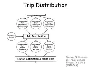
Travel Demand Forecasting: Trip Distribution. CE331 Transportation Engineering. Land Use and Socio-economic Projections. Trip Generation. Trip Distribution. Transportation System Specifications. Modal Split. Traffic Assignment. Direct User Impacts. Overall Procedure. Trip Distribution.

E N D
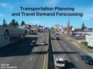
Travel Demand Forecasting:Trip Distribution CE331 Transportation Engineering
Land Use and Socio-economic Projections Trip Generation Trip Distribution Transportation System Specifications Modal Split Traffic Assignment Direct User Impacts Overall Procedure
Trip Distribution • Where to go? • Choice may vary with trip purpose • Input • Trips generated from and attracted to each zone (step 1 output) • Interzonal transportation cost (travel time, distance, out-of-pocket cost, …) • Output – trip interchange between zones • Presented as Origin-Destination (OD) matrix
Process • Allocate trips originating from each zone to all possible destination zones • Assume destination zones are competing with each other in attracting trips produced by zone i
Types of Models • Gravity Model • Trips are attracted to a zone as gravity “attracts” objects • Utility Maximization • Assumes that a traveler makes the decision that maximizes his/her utility
K-Factors • K-factors account for socioeconomic linkages not accounted for by the gravity model • Common application is for blue-collar workers living near white collar jobs (can you think of another way to do it?) • K-factors are i-j TAZ specific (but could use a lookup table – how?) • If i-j pair has too many trips, use K-factor less than 1.0 (& visa-versa) • Once calibrated, keep constant? for forecast (any problems here???) • Use dumb K-factors sparingly • Can you design a “smart” k factor? (TTYP)
Input data How do models compute this? See next pages… Does this table need to be symmetrical? Is it usually?
Convert Travel Times into Friction Factors Yes, but how did we get these?
Find the shortest path from node to all other nodes (from Garber and Hoel) 1 3 6 1 Here’s how … 1 2 3 4 4 2 2 1 3 2 2 5 6 7 8 3 1 2 1 3 3 4 9 10 11 12 3 1 2 1 4 4 4 13 14 15 16 Yellow numbers represent link travel times in minutes 3
STEP 1 1 3 6 1 1 2 3 4 4 2 2 1 2 3 2 2 5 6 7 8 3 1 2 1 3 3 4 9 10 11 12 3 1 2 1 4 4 4 13 14 15 16
STEP 2 1 4 3 6 1 1 2 3 4 4 2 2 1 2 5 3 2 2 5 6 7 8 3 1 2 1 3 3 4 9 10 11 12 3 1 2 1 4 4 4 13 14 15 16
STEP 3 1 4 3 6 1 1 2 3 4 4 2 2 1 2 5 3 2 2 5 6 7 8 4 3 1 2 1 4 3 3 4 9 10 11 12 3 1 2 1 4 4 4 13 14 15 16
STEP 4 1 4 3 6 1 1 2 3 4 Eliminate 4 2 2 1 5 >= 4 2 5 3 2 2 5 6 7 8 4 3 1 2 1 4 3 3 4 9 10 11 12 3 1 2 1 4 4 4 13 14 15 16
STEP 5 1 4 10 3 6 1 1 2 3 4 4 2 2 1 2 6 3 2 2 5 6 7 8 4 3 1 2 1 4 3 3 4 9 10 11 12 3 1 2 1 4 4 4 13 14 15 16
STEP 6 1 4 10 3 6 1 1 2 3 4 4 2 2 1 2 6 3 2 2 5 6 7 8 4 7 Eliminate 7 >= 6 3 1 2 1 4 7 3 3 4 9 10 11 12 3 1 2 1 4 4 4 13 14 15 16
STEP 7 1 4 10 3 6 1 1 2 3 4 4 2 2 1 2 6 3 2 2 5 6 7 8 4 3 1 2 1 4 7 3 3 4 9 10 11 12 8 Eliminate 8 >= 7 3 1 2 1 6 4 4 4 13 14 15 16
STEP 8 1 4 10 3 6 1 1 2 3 4 4 2 2 1 2 6 8 3 2 2 5 6 7 8 4 3 1 2 1 4 7 7 3 3 4 9 10 11 12 3 1 2 1 6 4 4 4 13 14 15 16
STEP 9 1 4 10 3 6 1 1 2 3 4 4 2 2 1 2 6 8 3 2 2 5 6 7 8 4 3 1 2 1 4 7 7 3 3 4 9 10 11 12 3 1 2 1 10 6 4 4 4 13 14 15 16
STEP 10 1 4 10 3 6 1 1 2 3 4 4 2 2 1 2 6 8 3 2 2 5 6 7 8 4 3 1 2 1 4 7 7 3 3 4 9 10 11 12 10 Eliminate 10 >= 7 Eliminate 3 1 2 1 10 6 4 4 4 13 14 15 16 10 10 >= 10
STEP 11 1 4 10 3 6 1 1 2 3 4 4 2 2 1 2 6 8 3 2 2 5 6 7 8 4 3 1 2 1 4 10 7 7 3 3 4 9 10 11 12 3 1 2 1 8 6 4 4 4 13 14 15 16 10
10 > 9 Eliminate STEP 12 1 4 10 3 6 1 1 2 3 4 9 4 2 2 1 2 6 8 3 2 2 5 6 7 8 4 3 1 2 1 10 >= 9 9 4 10 7 7 3 3 4 9 10 11 12 Eliminate 3 1 2 1 8 6 4 4 4 13 14 15 16 10
STEP 13 1 4 3 6 1 1 2 3 4 9 4 2 2 1 2 6 8 3 2 2 5 6 7 8 4 3 1 2 1 9 4 7 7 3 3 4 9 10 11 12 3 1 2 1 12 >= 10 12 8 12 6 4 4 4 13 14 15 16 10 Eliminate
STEP 14 1 4 3 6 1 1 2 3 4 9 4 2 2 1 2 6 8 3 2 2 5 6 7 8 4 3 1 2 1 9 4 7 7 3 3 4 9 10 11 12 3 1 2 1 12 >= 10 8 12 10 6 4 4 4 13 14 15 16 10 Eliminate
FINAL 1 4 1 2 3 4 9 2 6 8 5 6 7 8 4 9 4 7 7 9 10 11 12 8 10 6 13 14 15 16 10
Make sense? Calculate the Relative Attractiveness of Each Zone
First Iteration Distribution Advanced Concepts – not required for CE331
Comparing and Adjusting Zonal Attractions • Balanced attractions from trip generation = 76 • The gravity model estimated more attractions to TAZ 3 than estimated by the trip generation model. • What can we do? (see homework) Advanced Concepts – not required for CE331
Forecasting for Future Year Assignments • After successful base year calibration and validation (review … how?) • Use forecast land use, socioeconomic data, system changes • Forecasted production and attractions, and future year travel time skims • Apply gravity model to forecast year • Friction factors remain constant over time (what to you think?) In-class exercise Advanced Concepts – not required for CE331
A Simple Gravity Model tij = Pi Tj/(dijn Aj) Where Pi – trips generated from zone i; dij – distance or time; Tj – trips attracted to zone j; Aj – balancing factor; Aj =Σ (Pi /dijn) n – parameter.
Example – 1 • A new theater is expected to attract 700 trips from 2 zones with daily trip productions of 1500 and 3000. The distances to the new theater are 2 and 3 miles, respectively. The factor n is approximately 2. How many trips from each zone will be attracted to the theatre?
Example (cont’d) A1 = Σ (Pi /dijn) = (1500/22)+ (3000/32)= 708.3 t11=P1T1/(d112A1)=1500(700)/[22(708.3)]= 370.6 t21=P2T1/(d212A1)=3000(700)/[32(708.3)]=329.4
Utility Maximization • Consider travelers’ choice in trip-making decision • Use utility function (U) to reflect the attractiveness of an alternative (in this case, destination) • U = b0 + b1*z1 + b2*z2 + … + bn*zn • b0, b1, …: parameters • z1, z2, …: attributes of the alternative
Utility Maximization:Logit Model • Pr(i): probability of choosing alternative i over all other alternatives; • Ui: utility value of alternative (destination) i.