Forecasting Demand
220 likes | 466 Views
Forecasting Demand. Forecasting Methods. Qualitative – Judgmental, Executive Opinion - Internal Opinions - Delphi Method - Surveys Quantitative - Causal, Extrinsic Factors - Time Series. Causal Methods.

Forecasting Demand
E N D
Presentation Transcript
Forecasting Methods • Qualitative – Judgmental, Executive Opinion - Internal Opinions - Delphi Method - Surveys • Quantitative - Causal, Extrinsic Factors - Time Series
Causal Methods Seek Relation between Sales and Economic Indicators (Especially Leading Indicators) Example: Door Lock Demand & Housing Starts Month Housing Starts Door Locks January 4000 350 February 5000 450 March 3000 300 April 6000 550 May 7000 720
Time Series Forecasts Based on Past Demand Patterns or Components: • Average or Level • Trend • Seasonal • Cyclical (Omit) • Random (Cannot Forecast)
Time Series: Level Demand • Simple or Arithmetic Mean E.g. F5 = (103 + 121 + 130 + 150) / 4 = 126 • Moving Average – Discard Old Data • Weighted Average Ft+1 = t Dt + t-1Dt-1 +Etc. = Weight between 0 and 1, i = 1 D = Actual Demand t = Current Time Period (t=4) E.g. F5 = .4(150)+.3(130)+.2(121)+.1(103) = 133.5
Time Series: Level Demand Exponential Smoothing Weighted Average Ft+1 = Dt + (1-)Ft Ft is Old Forecast from Last Period E.g. F5 = (.2)(150) + (.8)(115) = 122
Time Series: Trends • Trend is Predictable Long Term Increase or Decrease in Demand • E.g. January 103 February 121 March 130 April 150 If Trend Continues, Averages are Too Low • Forecasting Techniques: - Regression (Least Squares) - Adjusted Exponential Smoothing
Time Series: Trends • Simple Regression: One Independent Variable E.g. Ft = a + bt (t is Time, a & b are Constants) F5 = 88.5 + (15)(5) = 163.5 • Multiple Regression: Multiple Independent Variables E.g. Ft = a + b1t + b2i (i is base index) F5 = 81 + (12.83)(5) + (16.67)(1.05) = 162.6 • We Can Use Excel to Get a & b’s
Time Series: Trends & Exponential Smoothing 1. Ft+1 = Dt + (1-)Ft = 122 2. Trend Factor = (Ft+1 – Ft) = 122 - 115 = 7 Tt+1 = (Ft+1 – Ft)+ (1- ) Tt = Weight between 0 and 1, Often = Tt = Old Trend, Use Trend Line Slope at First E.g. Tt+1 = .2(7) + .8(15) = 13.4
Time Series: Trends & Exponential Smoothing 1. Ft+1 = 122 • Tt+1 = .2(7) + .8(15) = 13.4 3. A Ft+1 = Ft+1 + (Lag)(Tt+1 ) Lag Can be (1/ ) = (1/.2) = 5 E.g. A Ft+1 = 122 + (5)(13.4) =189 Can You Do a Forecast for June?
Time Series: Seasonal Demand Seasonal Demand: Definite, Dependable Reason for Heavy Demand at One Time, Light Demand at Another 1. Construct Base Series or Index from Historical Demand • Divide All Demand by Appropriate Base • Forecast Using Any Method 4. Adjust Forecast by Multiplying by Appropriate Base
Evaluating Forecasts: MAD • MAD is Mean Absolute Deviation • Smaller the MAD, the Better • MAD = | Dt – Ft | / n Dt = Actual Demand Ft = Forecast n = Number of Periods
Evaluating Forecasts: MAD Example of MAD for May and June: Month Dt Ft | Dt – Ft | May 172 122 50 June 192 132 60 110 MAD = 110 / 2 = 55