Trip Distribution
Trip Distribution. Additional suggested reading: Chapter 5 of Ortuzar & Willumsen, third edition. November 2004. Trip Distribution Objectives. Replicate spatial pattern of trip making

Trip Distribution
E N D
Presentation Transcript
Trip Distribution • Additional suggested reading: Chapter 5 of Ortuzar & Willumsen, third edition November 2004
Trip Distribution Objectives • Replicate spatial pattern of trip making • Account for spatial separation among origins and destinations (proximity in terms of time, cost, & other factors) • Account for attractiveness among TAZs • Reflect human behavior
Destinations TAZ P 15 13 26 18 8 13 93 A 22 6 5 52 2 6 93 Origins 1 2 3 4 5 6 Sum T11 T12 T13 T14 T15 T16 O1 T21 T22 T23 T24 T25 T26 O2 T31 T32 T33 T34 T35 T36 O3 T41 T42 T43 T44 T45 T46 O4 T51 T52 T53 T54 T55 T56 O5 T61 T62 T63 T64 T65 T66 O6 D1 D2 D3 D4 D5 D6 1 2 3 4 5 6 Sum 1 2 3 4 5 6 Sum Trip Distribution • Convert Production and Attraction Tables into Origin - Destination (O - D) Matrices
Trip Distribution, Methodology • General Equation: • Tij = Ti P(Tj) • Tij = calculated trips from zone i to zone j • Ti = total trips originating at zone i • P(Tj) = probability measure that trips will be attracted to zone j • Constraints: • Singly Constrained • Sumi Tij = Dj OR Sumj Tij = Oi • Doubly Constrained • Sumi Tij = Dj AND Sumj Tij = Oi
Trip Distribution Models • Growth Factor / Fratar Model • Tij = Ti (Tj / T) • Tij = present trips from zone i to zone j • Ti = total trips originating at zone i • Tj = total trips ending at zone j • T = total trips in the entire study • Tij* = Tij (Fi Fj) / F • Fi = Ti* / Ti • Fj = Tj* / Tj • F = T* / T • * = estimated future trips
a Aj / Cij Trip Distribution Models You can consider this as the probability spatial distribution P(Tj) • Gravity Model • Tij = Ti • Tij = trips from zone i to zone j • Ti = total trips originating at zone i • Aj = attraction factor at j • Ax = attraction factor at any zone x • Cij = travel friction from i to j expressed as a generalized cost function • Cix = travel friction from i to any zone x expressed as a generalized cost function • a = friction exponent or restraining influence a Sum (Ax / Cix)
Trip Distribution Models • Intervening - Opportunities Model • Tij = Ti (e - e ) • Tij = trips from zone i to zone j • T = trip destination opportunities closer in time to zone i than those in zone j • Ti = trip end opportunities in zone i • Tj = trip end opportunities in zone j • L = probability that any destination opportunity will be chosen -LT -LT(T + Tj)
Model Advantages Disadvantages Growth Factor Gravity Intervening - Opportunities Simple Easy to balance origin and destination trips at any zone Specific account of friction and interaction between zones Does not require origin - destination data Claimed to bear a better “fit” to actual traffic Does not reflect changes in the frictions between zones Does not reflect changes in the network Requires extensive calibration Long iterative process Accounts for only relative changes in time - distance relationship between zones Arbitrary choice of probability factor Model Comparison New: Destination choice models build on intervening opportunities
Gravity Model Process • Create Shortest Path Matrix - Minimize Link Cost between Centroids • Estimate Friction Factor Parameters - Function of Trip Length Characteristics by Trip Purpose • Calculate Friction Factor Matrix • Convert Productions and Attractions to Origins and Destinations • Calculate Origin - Destination Matrix • Enforce Constraints on O - D Matrix - Iterate Between Enforcing Total Origins and Destinations
Shortest Path Matrix • Matrix of Minimum Generalized Cost from any Zone i to any Zone j (see OW p. 153) • Distance, Time, Monetary Cost, Waiting Time, Transfer Time, etc.. may be used in Generalized Cost • Time or Distance Often Used • Matrix Not Necessarily Symmetric (Effect of One - Way Streets) TAZ ID TAZ ID 1 2 3 4 5 6 C11 C12 C13 C14 C15 C16 C21 C22 C23 C24 C25 C26 C31 C32 C33 C34 C35 C36 C41 C42 C43 C44 C45 C46 C51 C52 C53 C54 C55 C56 C61 C62 C63 C64 C65 C66 1 2 3 4 5 6
Friction Factor Models • Exponential: • f(cij) = e c > 0 • Inverse Power: • f(cij) = cijb > 0 • Gamma: • f(cij) = a cij e a > 0, b > 0, c > 0 - c (cij) - b - b - c (cij) Trip Purpose a b c HBW 28507 0.020 0.123 HBP 139173 1.285 0.094 NHB 219113 1.332 0.010 ref. NCHRP 365 / TransCAD UTPS Manual pg. 80
Example friction factors using travel times alone Friction ij = 1/exp(-0.03* Timeij)
Friction Factor Matrices • Matrix of Friction from any Zone i to any Zone j, by Trip Purpose • Each Cell of a Friction Factor Matrix is a Function of the Corresponding Cell of the Shortest Path Matrix • Each Trip Purpose has a separate Friction Factor Matrix Because Trip Making Behavior Changes for Each Trip Purpose TAZ ID TAZ ID 1 2 3 4 5 6 F11 F12 F13 F14 F15 F16 F21 F22 F23 F24 F25 F26 F31 F32 F33 F34 F35 F36 F41 F42 F43 F44 F45 F46 F51 F52 F53 F54 F55 F56 F61 F62 F63 F64 F65 F66 1 2 3 4 5 6
Trip Conversion(Approximate) • Home Based Trips: Non - Home Based Trips: • Oi = (Pi + Ai) / 2 Oi = Pi • Di = (Pi + Ai) / 2 Di = Ai • Oi = origins in zone i (by trip purpose) • Di = destinations in zone i (bytrip purpose) • Pi = productions in zone i (by trip purpose) • Ai = attractions in zone i (by trip purpose) • Note: This Only Works for a 24 Hour Time Period • If our models are for one period in a day we prefer to work directly with Origins-Destinations
O - D Matrix Calculation • Calculate Initial Matrix By Gravity Equation, by Trip Purpose • Each Cell has a Different Friction, Found in the Corresponding Cell of the Friction Factor Matrix • Enforce Constraints in Iterative Process • Sum of Trips in Row i Must Equal Origins of TAZ i • If Not Equal, Trips are Adjusted Proportionally • Sum of Trips in Column j Must Equal Destinations of TAZ j • If Not Equal, Trips are Adjusted Proportionally • Iterate Until No Adjustments Required
Destinations Origins 1 2 3 4 5 6 Sum T11 T12 T13 T14 T15 T16 O1 T21 T22 T23 T24 T25 T26 O2 T31 T32 T33 T34 T35 T36 O3 T41 T42 T43 T44 T45 T46 O4 T51 T52 T53 T54 T55 T56 O5 T61 T62 T63 T64 T65 T66 O6 D1 D2 D3 D4 D5 D6 1 2 3 4 5 6 Sum O - D Matrix Example:
Aj / frictionij Gravity model probability Sum (Ax / frictionix)
Trip Interchange - iteration 1 For each cell value we apply the gravity equation once - in this iteration - after this we use the ratio to adjust the values in the cells - until row and column targets are satisfied - see also OW - chapter 5
Trip interchange - iteration 2 Using the ratios from before we succeed in getting the targets for the sums of cells for each column - look at the other ratios
Trip interchange - iteration 4 We get both rows and columns to produce the sums we want!
Multiple Matrices • For each trip purpose obtain different Origin-Destination Tij matrices • Usually these are 24 hour Matrices (number of trips from one zone to another in a 24 hour period) • In assignment we will need a matrix of vehicles moving from a zone to another during a specific period (peak usually) in a typical day
Final O - D Matrix (simplified) • Combine (Add) O - D Matrices for Various Trip Purposes • Scale Matrix for Peak Hour • Scale by Percent of Daily Trips Made in the Peak Hour • 0.1 Often Used (10% of daily trips) • Scale Matrix for Vehicle Trips • Scale by Inverse of Ridership Ratio to Convert Person Trips to Vehicle Trips • 0.95 to 1 Often Used • Note: Mode Split Process / Models More Accurate, - we will explore them in class