Download
1 / 47
490 likes | 1k Views
Land Use and Travel Demand Forecasting. CE 451/551 Sources: National Highway Institute Workshop on Travel Demand Forecasting Chapter 4, Meyer and Miller’s Urban Transportation Planning, Ch. 6, and Dr. Paul Hanley, University of Iowa

E N D
Land Use and Travel Demand Forecasting CE 451/551 Sources: National Highway Institute Workshop on Travel Demand Forecasting Chapter 4, Meyer and Miller’s Urban Transportation Planning, Ch. 6, and Dr. Paul Hanley, University of Iowa See also: INCORPORATING LAND USE AND ACCESSIBILITY VARIABLES IN TRAVEL DEMAND MODELS, by Chuck Pervis
Pop quiz • Define the word “sensitive” as it relates to models and policies
Objectives • Describe land use estimates and how they are used in the context of TDF • Identify factors influencing household and employment location • Identify methodologies for forecasting the location of households and employment • Describe sub-allocation
Terminology • Demographic data and projections • Socioeconomic data and projections • Land use estimates • Population • Households • Employment • Sub-allocation
Key Concepts What is land use? In travel forecasting terms, land use refers to: • Number, type and location of households • Number, type and location of employment • Additional socioeconomic data
Why are we interested • Land use estimates are a major input to the TDF process • Bad estimates cannot be corrected later in the TDF process • Land use forecasts must be reasonable for results of TDF and emissions estimates to be reasonable • Land use policies and projects are seen increasingly as transportation solutions – model must be sensitive
Not from NHI What is the land use/ transportation relationship? • Effect of one on the other? • Integrated? Why not? • Different “departments” (e.g., energy problem policy solution) • Typical: Mode choice • Typical: Vehicle improvement • What about land use change? • Different analytical techniques • Internal inconsistencies • trip dist from LU model ≠ trip dist from TDF model • Network used in LU model ≠ network in TDF model • LU modeling not done much in USA 1970-1990s (but resurgence is underway)
Data sources • Census • CTPP • State Employment Commission • Market research listings • Local area population and employment data • Telephone directory • Aerial photos • State Dept. of Finance • Local Planning departments
Base year estimates • For model calibration/base year, obtain most recent population, household and employment estimate • Sub-allocate estimates to TAZs (if not already at this level) • Output: Household and employment estimates by TAZ • Classify estimates by household size, income, employment type • Use in the TDF process
Future year estimates • Control totals • Usually, land use forecasts assume a “control total” for the region or sub-region • These forecasts are usually developed by a state economic development or employment agency • In many states, regions must use these totals to constrain their forecasts • See census state population forecasts here
Future year estimates • Start with regional forecast from state • Growth in population, households by income class, household size and employment by type sub-allocated to TAZs • Issues • Complicated technical steps • Political involvement
Population Forecast • Ratio-trend method • Cohort survival method (pop + birth - death + immigration- emigration) • Economic-base method • Constant or gradually declining compound growth rate • Constant absolute rate change over a fixed period
Employment Forecast • Trend extrapolation • Input-output analysis • Judgment estimation
Sub-allocation • Forecasts, and sometimes base year estimates, need to be sub-allocated from regional and district totals to TAZs
What factors do you think are important location considerations? • for a commercial landuse? • an industrial land use? • a residential land use?
Location choice considerations • Commercial/industrial • Transportation access to labor, customers, suppliers and shipping • Cost and tax of site • Local zoning regulation • Residential • Housing stock and cost • Quality of schools, shopping, parks and entertainment • Transportation access to work, shopping, and other activities
Forecasting techniques • Qualitative methods • Delphi or expert panel • Committees (policy, technical) • Comprehensive plans • Quantitative methods • Logit models (draws on random utility theory and discrete choice analysis as their theoretical base) • Input output models (e.g. Implan, Rims-II) • Gravity* models (derived from Lowry model) *similar to, but not the same as the trip distribution gravity model
35 largest MPOs … • Twelve MPOs are using DRAM-EMPAL models • Five MPOs are using their own models (POLIS, PLUM, and three local models) • One MPO is in the process creating its own model • Two MPOs use the Delphi (exchange of expert opinion) Technique Source: “Review of Land Use Models: Theory and Application,” Kazem Oryani, URS Greiner, Inc. and Britton Harris, University of Pennsylvania http://ntl.bts.gov/lib/7000/7500/7505/789761.pdf
Qualitative method: Delphi • Systematic way to utilize expert opinion • Broad range of experts • Begins with questionnaire • Anonymous participation with statistical group response • More than one round of questions and answers • Moderator facilitates discussion • Advantages: • Time and cost savings • Diversity of experts • Limitations: not able to reflect complex real world interactions Click here for e-version of book
The Lowry Model • Pittsburg 1964 • Growth is a function of the “basic” sector • employment that meets non-local demand • Location not critical (for “export”) • exogenous (must be given) • Retail sector (services) • Endogenous • Multiple of basic sector • Residential sector (function of basic and retail) – also endogenous • Location of retail and residential a “gravity” function of distance to jobs in the basic sector source: , Rodrigue, J-P et al. (2006) The Geography of Transport Systems, Hofstra University, Department of Economics & Geography, http://people.hofstra.edu/geotrans/eng/ch6en/meth6en/ch6m2en.html
Lowry Model (cont.) Economic forecast Location of industrial employment Friction of space Location of industrial employees’ residences Location of service employment Friction of space Location of service employees’ residences source: , Rodrigue, J-P et al. (2006) The Geography of Transport Systems, Hofstra University, Department of Economics & Geography, http://people.hofstra.edu/geotrans/eng/ch6en/meth6en/ch6m2en.html
Lowry Model (cont.) source: , Rodrigue, J-P et al. (2006) The Geography of Transport Systems, Hofstra University, Department of Economics & Geography, http://people.hofstra.edu/geotrans/eng/ch6en/meth6en/ch6m2en.html
Lowry Model Steps • The spatial distribution of basic employment is assumed as given. • The location of the basic workers is determined according to a location-probability matrix, itself the result of a least friction of distance function. • Calculation of the residential sector per zone according to the population per worker multiplier. • Calculation of the number of non-basic workers per zone to service the population. This is the result of a non-basic worker per capita multiplier. • The location of non-basic workers is determined according to a location-probability matrix. • Revision of the total population according to the population per worker multiplier. • Calculation of the total number of workers and the total population. This is the summation of the basic and non-basic employment and of the basic and non-basic related population. • The above processes (4 to 7) are repeated until a convergence is reached, that is an optimization of the equation system of the model following a set of constrains such as density. source: , Rodrigue, J-P et al. (2006) The Geography of Transport Systems, Hofstra University, Department of Economics & Geography, http://people.hofstra.edu/geotrans/eng/ch6en/meth6en/ch6m2en.html
Lowry Equations (singly constrained) source: , Rodrigue, J-P et al. (2006) The Geography of Transport Systems, Hofstra University, Department of Economics & Geography, http://people.hofstra.edu/geotrans/eng/ch6en/meth6en/ch6m2en.html
Lowry variable definitions Tij = Interaction from residential zone i to work zone j (work-related travel). Sij = Interaction from residential zone i to service zone j (service-related travel). Pi = Total population of a zone i. Ei, EBi and ESi = Total employment, employment in the basic (B) and service (S) sectors for zone i. dij = Euclidean distance between zone i and j (in km). Alpha = population over basic employment multiplier. Beta = service employment over population multiplier. Lambda: Friction factor for residential interactions. Micron: Friction factor for services interactions. WTTRij and WTTSij = Willingness to travel for Residential (R) or Services (S) between zone i and j. LPRij and LPSij = Locational probability for Residential (R) or Services (S) between zone i and j. Prof. Rodrique’s Operational Lowry Model Spreadsheet source: , Rodrigue, J-P et al. (2006) The Geography of Transport Systems, Hofstra University, Department of Economics & Geography, http://people.hofstra.edu/geotrans/eng/ch6en/meth6en/ch6m2en.html
Lowry limitations • Static model – evolution of transport system not considered • Service jobs are the big changes these days • No freight • More recent variants do these things (see pages to follow) source: , Rodrigue, J-P et al. (2006) The Geography of Transport Systems, Hofstra University, Department of Economics & Geography, http://people.hofstra.edu/geotrans/eng/ch6en/meth6en/ch6m2en.html
“DRAM/EMPAL” • Derived from the Lowry Gravity Model • Two main components • Disaggregated Residential Allocation Model (DRAM) • Employment Allocation Model (EMPAL) • Allows interactions between land use and transportation • Forecasts household location based on employment and work trips between zones • Inputs • employment, households, vacant land, % land developed, regional employment>households matrix, zonal trip impedance matrix • Most widely used model in the US • has been applied in Atlanta, Chicago, Dallas, Houston, Los Angeles, Sacramento, Boston, Detroit, Kansas City, Phoenix, San Antonio, Seattle, and Orlando.
Integrated Land Use and Transportation Package Trip Generation Household location DRAM Trip Distribution Employment location EMPAL Modal Split Economic forecast Traffic Assignment Friction of space source: , Rodrigue, J-P et al. (2006) The Geography of Transport Systems, Hofstra University, Department of Economics & Geography, http://people.hofstra.edu/geotrans/eng/ch6en/meth6en/ch6m2en.html
“METROPILUS” (DRAM/EMPAL/LANDCON) • DRAM/EMPAL: can be used to produce • employment location forecasts that reflect changes in the location of households • household location forecasts that reflect changes in the location of employers. • LANCON (for LANd CONsumption) • Input: calculated demands for residential and employment uses by zone • estimates the change in each land use category • 100-300 zones (each can contain 6,000 - 10,000 people) • Four - eight household types specified by income and place of residence • Four - eight employment types, located by place of employment • purchased as part of a comprehensive consulting package $$$ • See: Literature Review for Urban Growth modeling and Environmental Impact Analysis
“Index” • Gravity-type • introduced by Criterion in 1994 • functions as a GIS-based neighborhood to regional scenario builder • Cost $ • Reference: Criterion Planners (software home page)
MEPLAN • Derived from Lowry model, focus on housing market (bid-rent) and LOGIT type • Integrated software package (demand and supply of both land use and transportation) • Compares the effects of changes in various public policies • Three main functions • determines effects of transport on the choices of location by residents, employers, developers, and others • determines how land use and economic activity create the demand for transport • projects and evaluates the many impacts that planning decisions will have on land use and transport • Applied in • Cambridge and Stevenage, U.K.; Santiago, Chile: Sao Paulo, Brazil; Tehran, Iran; Bilbao, Spain; Helsinki, Finland; Tokyo, Japan
MEPLAN • Suggested staff: transport engineer, planner, and economist • Cost $$ • References • NCHRP Project 8-32, Task 3 (1998). “Land Use Impacts of Transportation: A Guidebook.” Prepared By: Parsons Brinckerhoff Quade & Douglas, Inc., pp. 63-70. • United States Environmental Protection Agency (2000). “Projecting Land-Use Change: • A Summary of Models for Assessing the Effects of Community Growth and Change on Land-Use Patterns.” Office of Research and Development, pp. 86-90. • A review of the MEPLAN modelling framework from a perspective of urban economics
MEPLAN Transportation / Land Use Model Rents Non-Exporting Employment and Total Population Employment and Residences Locations and Trips Trip Distribution Exporting Industry Employment Forecast Modal Choice Traffic Assignment Friction of Space
MEPLAN “MEPLAN land use and transportation-interaction models traditionally include models of business-location choice. The mechanisms in the model that allow for realistic aggregate assignment of firms to zones, and the resulting impact that firm location has on the entire modeling system, are described. The models use a form of logit function to allocate production activities to zones. Interdependencies in the Social Accounting Matrix, together with trip- and land-cost data and usage rates, generate a utility function for the attractiveness of purchasing a given sector's output from a given zone. The alternative specific constants and the dispersion parameter are estimated in calibration, based primarily on cost data, trip-length distributions, and arrangement of activity in a calibration year. Results from a model of Sacramento show the various features and strengths of the model, while pointing out some weaknesses and potential pitfalls. The strengths include the realistic representation of current and continuing patterns, the close linkages between different industry and household types, and the market-based nature of the model. The weaknesses include the aggregate nature of the model and the possibility of difficulties in establishing realistic, alternative, specific constants.” Source: FIRM LOCATION IN THE MEPLAN MODEL OF SACRAMENTO , Abraham, J E Transportation Research Record No. 1685
Internet Planning for Community, Energy, Economic and Environmental Sustainability (PLACE3s) • LOGIT-type • ArcView (GIS) platform • used by Sacramento Council of Governments (SACOG) • Blueprint: tool that uses PLACE3S in conjunction with the MEPLAN model and SACMET (Sacramento’s travel demand model) • can be run on the internet for no charge? • Blueprint description • Blueprint Power Point
TRANUS • LOGIT-type • Integrated Land Use and Transport Planning System • Simulates effects of projects and policies relating to location of activities, land use, and the transportation system • Evaluates effects from economic, financial and environmental points of view • applied in Baltimore, MD and Salem, OR • Cost $ • References • United States Environmental Protection Agency (2000). “Projecting Land-Use Change: A Summary of Models for Assessing the Effects of Community Growth and Change on Land-Use Patterns.” Office of Research and Development, pp. 117-124. • developer’s website
UrbanSIM • LOGIT-type • behavioral approach • Treats urban development as the interaction between market behavior and governmental actions • simulates • where households and businesses choose to locate • how governments place constraints on development in the form of land use plans and policies • Cost: free and downloadable from http://www.urbansim.org. • still in developing stages • experience in Honolulu, HI, Eugene-Springfield, OR, Salt Lake City, UT, and Seattle, WA. • requires • GIS tools • statistical packages, like SAS or SPSS for calibration • LOGIT estimation software package • integration with a travel model to reflect transportation through accessibility measures contained in the model • References • NCHRP Project 8-32, Task 3 (1998). “Land Use Impacts of Transportation: A Guidebook.” Prepared By: Parsons Brinckerhoff Quade & Douglas, Inc., pp. 89-95. • United States Environmental Protection Agency (2000). “Projecting Land-Use Change: A Summary of Models for Assessing the Effects of Community Growth and Change on Land-Use Patterns.” Office of Research and Development, pp. 134-139 • Slide Show
What if? • Lowry Gravity-type • ESRI GIS based • model changes that may result from different policy strategies References • Klostermann, Richard. (1998) The What if? Collaborative Planning Support System. Environment and Planning, B: Planning and Design, 26 (1999): 393-408 • What if?, Inc
Validation and Error Checking • Document procedures and results • Check output data against independent data (trends) • Households • Auto availability • Income • Total employment • Special generators • Illustrate output data