Download
1 / 38
400 likes | 621 Views
Quad Modeling 101. Riki Conrey Indiana University (with some tinkering by Jeff Sherman, UC Davis)

E N D
Quad Modeling 101 Riki Conrey Indiana University (with some tinkering by Jeff Sherman, UC Davis) Conrey, F. R., Sherman, J. W., Gawronski, B., Hugenberg, K., & Groom, C. (in press). Separating multiple processes in implicit social cognition: The Quad-Model of implicit task performance. Journal of Personality and Social Psychology.
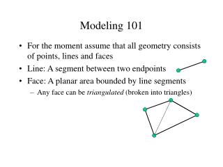
Multinomial models are processing trees Each parameter is a probability Probabilities later in the tree are conditional on the probabilities before them Conditional probabilities are combined using multiplication Things you have to know
Defining the parameters Association ACtivation 1 - AC Either the association is activated (AC), or it’s not (1 – AC) Note that these probabilities sum to 1, the total possible probability
Discriminable Association ACtivation 1 - D 1 - AC If the association is activated (AC), then the answer might be discriminable (D) or it might not (1-D). Discriminability simply measures the likelihood that the correct answer could be determined. If the association is activated, and the item is discriminable, the probability is expressed AC * D If the association is activated, and the item is not discriminable, the probability is expressed AC * (1-D)
Discriminable Association ACtivation 1 - D 1 - AC Discriminable 1 - D Items can be discriminable even if the association is not activated (1-AC) Again, if the association is not activated, and the item is discriminable (1-AC) * D If it’s not discriminable (1-AC) * (1-D) In the Quad-Model, D is set equal across AC and 1-AC. Obviously, this means that discriminability is independent of association activation.
Overcoming Bias Discriminable 1 - OB Association ACtivation 1 - D 1 - AC Discriminable 1 - D If the association is activated (AC), and the item can be discriminated (D), then you have to pick one. The probability of overcoming the associative bias is (OB), and the probability of the event is AC * D * OB The probability that you don’t overcome the bias is AC * D * (1-OB) Of course, AC and D are in conflict only on incompatible blocks
Overcoming Bias Discriminable 1 - OB Association ACtivation 1 - D 1 - AC Discriminable 1 - D Guess Right One more: If there’s no association (1-AC), and the item’s not discriminable (1-D), then you have to guess one answer. In the Quad model, (1-AC) * (1-D) * G, means you guess the answer on the right. (1-AC) * (1-D) * (1-G) means you guess the answer on the left. 1 - G
Obviously, we can make up as many imaginary processes as we want to. But in order to actually estimate the values of real probabilities, we need to connect them to observable probabilities. The Quad-Model uses observed probabilities of correct and incorrect responses on the IAT (and other measures) to estimate parameters. Linking the tree to observable responses
Compatible, Right + OB + 1-OB D + 1-D AC 1-AC D + + 1-D G - 1-G This is the whole point: Each of these paths predicts a specific response. Imagine that on a compatible trial, the stimulus should be assigned to the right-hand key. In this case, you’ll get the answer right no matter what you do, except if you have no association, no discriminability, and you guess left (1-AC) * (1-D) * (1-G)
Incompatible, Right Let’s walk through it. On an incompatible, right-hand trial (e.g. “Rainbow”), the association is activated with the probability AC. If that happens, then you are able to figure out the correct answer with the probability D. If both of these things are true, and you overcome your bias (OB), you’ll discriminate the answer and produce the correct response. + OB 1-OB D 1-D AC 1-AC D 1-D G 1-G So, if AC and D and OB, then correct response, right? Formally, AC and D and OB, is simply AC * D * OB.
Incompatible, Right If you have the association, and you can discriminate the answer, but you don’t overcome the bias, you’ll get the answer wrong. That’s because the correct response on this incompatible trial is to pair Pleasant with Black, but the association drives you to pair Pleasant with White. + OB - 1-OB D 1-D AC 1-AC D 1-D G 1-G So far, then, we know that AC * D * OB leads to a correct response, and AC * D * (1-OB) leads to an incorrect response
Incompatible, Right But there’s more than one way to get an incorrect response. Say that the association is activated (AC), but you couldn’t explicitly determine the answer (1-D). Then there’s no competition and no overcoming, you just respond in line with the bias and get the answer wrong. + OB - 1-OB D - 1-D AC 1-AC D 1-D G 1-G So AC * D * (1-OB) leads to an incorrect response Or AC * (1-D) also leads to an incorrect response
Incompatible, Right If the opposite happens—no association is activated (1-AC) and discrimination is possible (D)—then you discriminate the answer and get it right. If there’s no association and no discriminability, then either you guess the response on the right (G) and get it right, or the response on the left (1-G) and get it wrong. + OB - 1-OB D - 1-D AC 1-AC D + 1-D G + 1-G -
Incompatible, Right So we have a set of six equations: + OB AC * D * OB AC * D * 1-OB AC * (1-D) (1-AC) * D (1-AC) * (1-D) * G (1-AC) * (1-D) * (1-G) - 1-OB D - 1-D AC 1-AC D + 1-D G + 1-G - We need to combine them in some way that relates these invisible parameters to our observable correct and incorrect responses.
Remember that when you’re talking about the probabilities of several events all happening, you combine them with and, otherwise known as multiplication When you’re talking about any of several events occurring, you combine them with or, otherwise know as addition Predicting responses from parameters
Incompatible, Right + OB - 1-OB D - 1-D AC 1-AC D + 1-D G + 1-G - So the total probability of a correct response is AC * D * OB + (1-AC) * D + (1-AC) * (1-D) * G That is, the first probability or the second or the third.
Incompatible, Right + OB - 1-OB D - 1-D AC 1-AC D + 1-D G + 1-G - The total probability of an incorrect response is AC * D * (1-OB) + AC * (1-D) + (1-AC) * (1-D) * (1-G) If you add the equations for correct and incorrect responses together, you get 1.
Estimating parameter values That little “|” character means “given” in probability speak p(correct| incompatible, right) = AC * D * OB + (1-AC) * D + (1-AC) * (1-D) * G p(incorrect| incompatible, right) = AC * D * (1-OB) + AC * (1-D) + (1-AC) * (1-D) * (1-G) These are our equations. Try solving for the parameters…
p(correct| incompatible, right) = AC * D * OB + (1-AC) * D + (1-AC) * (1-D) * G p(incorrect| incompatible, right) = AC * D * (1-OB) + AC * (1-D) + (1-AC) * (1-D) * (1-G) Of course, you can’t. Seventh grade math showed us that if you have four variables and two equations, you have a big pile of nothing. Or at least, you cannot solve for specific values. Thank goodness, the incompatible, right correct and incorrect responses are not the only ones we observe in the IAT.
p(correct| compatible, right) p(incorrect| compatible, right) p(correct| compatible, left) p(incorrect| compatible, left) p(correct| incompatible, right) p(incorrect| incompatible, right) p(correct| incompatible, left) p(incorrect| incompatible, left) p(correct| practice, right) p(incorrect| practice, right) p(correct| practice, left) p(incorrect| practice, left) Hooray, we’re rich in categories! Wait! These need to be independent probabilities. If I know the probability of a correct response, the probability of the incorrect response is not independent of that. This will become important when we fit the model Response categories
Full model and all the categories Incompatible Compatible Left Left Right Right + + + + OB - - + + 1-OB D Practice - - + + Left Right 1-D AC 1-AC D + + + + + + 1-D G + - + - + - 1-G - + - + - + Here are the predicted responses. I’m not going to write every equation here, but all the equations can be deduced from this diagram, and they’re in the model template file.
At this point, it’s a good idea to get out the model template file. You’ve already probably imagined how we get the parameters. We “solve” the equations to get the values. But because these models are overconstrained, that is, there is no one to one correspondence between categories and parameters, we use maximum likelihood estimation (MLE) to best guess the parameter values. It is not very interesting to show that a fully saturated model (i.e., one that has a separate parameter for each type of response) can fit the data. Of course it can. You must have fewer parameters than categories of responses. Fitting the Quad-Model
The hard part of multinomial modeling is specifying the model. That means you can’t estimate all four parameters for each possible response type. You have to constrain parameters to stay equal when they should not vary. Then you can look at interesting, meaningful differences. The Quad-Model estimates the following 6 parameters separately. 2 AC parameters— AC flowers-pleasant AC insects-unpleasant 2 OB parameters— OB attributes OB targets 1 D parameter 1 G parameter Note: The model also can be fit with a single OB parameter (see model templates). This allows modeling to be achieved without relying on the practice trials (which can be problematic). The one OB model often provides better model fit. Specifying the model
In the upper left-hand corner of the demo excel file, you should see the six parameter names with values to the right. These values vary between 0 and 1 MLE mushes the values around until the model provides the best overall fit to the observed data.
Fit We measure model fit with a chi-square statistic. The chi-square measures the difference between the actual counts of correct and incorrect responses and the predicted counts estimated by the parameter equations. These are the totals of correct and incorrect responses that the participants make. These are the chi-squares that compare the actual and predicted counts. These are the probabilities estimated by the parameters. You get these from the equations we discussed earlier. They’re linked to the parameters in column B.
Getting Excel to fit the model Now you have to use Solver. If you don’t have the add-in installed, go to ToolsAdd-Ins and install it. If it’s already installed go to ToolsSolver Solver is changing the parameter values to minimize the chi-square. It is good to have the parameter values in B set to .5 for this.
Fit The fit of the whole model is the sum of all the category chi-squares. Smaller chi-squares are better. You want the fit to be non-significant!!!! This is because you don’t want the actual and predicted responses to be different. You want the model to accurately describe the data.
Degrees of freedom So you want it non-significant, but how do you know? You need degrees of freedom for the model. In modeling Degrees of freedom = Uniquely predicted categories - Parameters Let’s begin by counting categories. The demo file has 16 categories. But half of those are not uniquely predicted (errors and non-errors are the same). So the demo file has 8 uniquely predicted categories. And 6 parameters So 8 – 6 = 2 degrees of freedom.
Degrees of freedom If you don’t intend to change the models or mess around with them in any way, that’s all you need to know. Skip ahead. But…it’s not all there is. Wait, you say to yourself, where did all the categories go? The compatible block has four item types! It does, but the responses for flowers and pleasant items and insects and unpleasant items are predicted by exactly the same equations. They’re not unique. So we sum those responses because the model predicts that they are produced through the same processes.
Degrees of freedom If you re-specify the model so that there are more or fewer parameters, you have to be aware of which categories are uniquely predicted by the specification. Setting things equal does not always increase your degrees of freedom Allowing parameters to vary sometimes gives you more degrees of freedom If you mess around with the model specification, you have to make sure your new model is identifiable, that is, that one set of error rates only produces one set of parameters. I’m not going to get into how to do this mathematically, but it can be difficult. However, a simple way to prove identifiability is to run the model more than once for the same data set with different start values for the parameters. If you get the same results, you have good evidence that the model is identifiable.
So you have a chi-square And you have degrees of freedom And you have a p-value If p>.05, the model fits. Interpreting model fit
Next, you have to figure out what your parameters mean (i.e., establish construct validity). Hypothesis testing can help you do that. Test a hypothesis by setting two or more parameters equal. The change in the chi-square shows you how much the change affects the model fit. If it’s lots, then the parameters are different and can’t be set equal. Formally, the chi-square for the test is equal to the change in chi-square. Df is equal to the number of parameters saved (1 if you’re setting 2 parameters equal). You want p<.05. You want the model fit to change significantly. Hypothesis testing
Getting Excel to test hypotheses Open solver and add a constraint that sets your parameters equal. Here, I’m setting AC Insect-unpleasant (B2) equal to AC Flower-pleasant (B3). χ2 for the whole model = 1.74 χ2 for the new model = 11.21 Δ χ2 = 9.47 Df for the test = 1 So the test: χ2 (1) = 9.47, p = .002 These parameters are significantly different. That means that the negative and positive associations for Insects and Flowers, respectively, differ in strength.
Let’s say we want to fit different conditions. The second sheet of the model demo gives an example. Imagine that we have 2 conditions, one with a response window, and one with no response window To model both conditions simultaneously, follow exactly the same procedure as the first model, just split your data by condition. Doing this shows that the model fits within each condition, and overall, across conditions (see cells B53 & B56) Comparing conditions
Hypotheses then can be tested across the conditions (set D in the Window condition equal to D in the No Window condition). Setting D equal across conditions increases the Chi-square value of the whole model from 4.39 to 37.31. This is a significant loss of model fit. Thus, D is significantly greater in the No Window than in the Window condition. Hypothesis Testing Across Conditions
Fitting models relies on accepting the null Fitting models also relies on chi-square, which is sensitive to small cell sizes That means you need a lot of observations Power and comparing conditions
No. But it’s enough to get you started. You will find out all kinds of stuff as you go along. Reliable individual estimates require many errors per subject REMEMBER Feel free to mess around with the model structure (it’s fun), but whatever you come up with needs to be identifiable and have the correct number of degrees of freedom. Is that it?
Get Quad-Modeling. You’ll get the hang of it really fast, and it’s really fun. When you run into trouble, you can e-mail me at jsherman@ucdavis.edu or rconrey@indiana.edu I am not an expert in multinomial modeling. You should definitely check out the work of Batchelder, Riefer, and Klauer. You’re ready!