Download
1 / 24
240 likes | 257 Views
Pipelining. Adding registers along a path split combinational logic into multiple cycles each cycle smaller than previously increase throughput. Pipelining. Delay, d, of slowest combinational stage determines performance Throughput = 1/d : rate at which outputs are produced

E N D
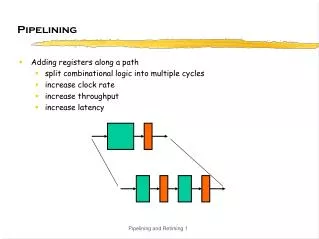
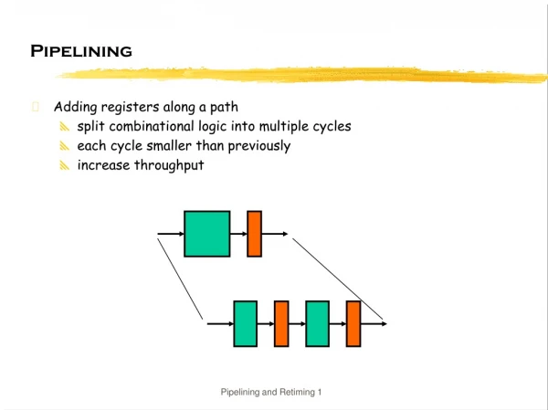
Pipelining • Adding registers along a path • split combinational logic into multiple cycles • each cycle smaller than previously • increase throughput Pipelining and Retiming 1
Pipelining • Delay, d, of slowest combinational stage determines performance • Throughput = 1/d : rate at which outputs are produced • Latency = n•d : number of stages * clock period • Pipelining increases circuit utilization • Registers slow down data, synchronize data paths • Wave-pipelining • no pipeline registers - waves of data flow through circuit • relies on equal-delay circuit paths - no short paths Pipelining and Retiming 2
When and How to Pipeline? • Where is the best place to add registers? • splitting combinational logic • overhead of registers (propagation delay and setup time requirements) • Example: 16-bit adder, add 8-bits in each of two cycles • What about cycles in data path? Pipelining and Retiming 3
Retiming • Process of optimally distributing registers throughout a circuit • minimize the clock period • minimize the number of registers Pipelining and Retiming 4
Retiming (cont’d) • Fast optimal algorithm (Leiserson & Saxe 1983) • Retiming rules: • remove one register from each input and add one to each output • remove one register from each output and add one to each input Pipelining and Retiming 5
Example - Digital Correlator • yt = d(xt, a0) + d(xt-1, a1) + d(xt-2, a2) + d(xt-3, a3) • d(xt, a0) = 0 if x a, 1 otherwise (and passes x along to the right) yt + + + host d d d d a0 a1 a2 a3 xt Pipelining and Retiming 6
+ + + host d d d d Example - Digital Correlator (cont’d) • Delays: adder, 7; comparator, 3; host, 0 cycle time = 24 Pipelining and Retiming 7
+ + + host d d d d + + + host d d d d Example - Digital Correlator (cont’d) • Delays: adder, 7; comparator, 3; host, 0 cycle time = 24 cycle time = 13 Pipelining and Retiming 8
a D Q c a x D Q x b d d b D Q a D Q a x D Q b x b D Q D Q c c D Q Retiming examples • Shortening critical paths • Create simplification opportunities Pipelining and Retiming 9
Optimal Pipelining • 1) Add registers 10 13 7 8 6 5 10 13 7 8 6 5 Pipelining and Retiming 10
Optimal Pipelining • 2) Use retiming to find optimal location 10 13 7 8 6 5 Pipelining and Retiming 11
Systolic Arrays • Set of identical processing elements • specialized or programmable • Efficient nearest-neighbor interconnections (in 1-D, 2-D, other) • SIMD-like • Multiple data flows, converging to engage in computation Analogy: data flowing through the system in a rhythmic fashion – from main memory through a series of processing elements and back to main memory Pipelining and Retiming 12
Example - Convolution • yj = xjw1 + xj+1w2 + . . . + xj+n-1wn - x3 - x2 - x1 w4 w3 w1 w2 - - - y1 - y2 - y3 - y1 = x1w1 + x2w2 + x3w3 + x4w4 y2 = x2w1 + x3w2 + x4w3 + x5w4 y3 = x3w1 + x4w2 + x5w3 + x6w4 . . . . Pipelining and Retiming 13
Example - Convolution (cont’d) w4 w3 w2 w1 x6 – x5 – x4 – x3 – x2 – x1 – – – y1 – y2 – y3 x6 – x5 – x4 – x3 – x2 – x1 – – – y1 – y2 – y3 x6 – x5 – x4 – x3 – x2 – x1 – – – y1 – y2 – y3 x6 – x5 – x4 – x3 – x2 – x1 – – – y1 – y2 – y3 x6 – x5 – x4 – x3 – x2 – – – y1 – y2 – y3 x6 – x5 – x4 – x3 – x2 – y1 – y2 – y3 x6 – x5 – x4 – x3 – y1 – y2 – y3 x6 – x5 – x4 – x3 – y2 – y3 Pipelining and Retiming 14
Convolution - Another Look • Repeated vector product ……x9……x8……x7……x6……x5……x4……x3……x2……x1……x0 * * * * w3 w2 w1 w0 y3 = Pipelining and Retiming 15
* + * + * + * + Convolution Example x7 x6 x5 x4 x3 x2 x1 x0 w3 w2 w1 w0 y0 0 Pipelining and Retiming 16
* + * + * + * + Convolution Example x7 x6 x5 x4 x3 x2 x1 w3 w2 w1 w0 y1 0 Pipelining and Retiming 17
* + * + * + * + 0 Pipelining and Retiming 18
* + * + * + * + 0 Pipelining and Retiming 19
* + * + * + * + x5 x7 x6 x4 x1 x3 x2 x0 w3 w2 w1 w0 0 Pipelining and Retiming 20
c11 c12 c13 c14 c21 c22 c23 c24 c31 c32 c33 c34 c41 c42 c43 c44 Example: Matrix Multiplication • C = A B cij = k=1n aikbkj Pipelining and Retiming 21
Example: Matrix Multiplication |||b44 ||b43 b34 |b42 b33 b24 b41 b32 b23 b14 b31 b22 b13 | b21 b12 || b11 ||| c11 c12 c13 c14 c21 c22 c23 c24 c31 c32 c33 c34 c41 c42 c43 c44 – – – a14 a13 a12 a11 – – a24 a23 a22 a21 – – a34 a33 a32 a31 –– a44 a43 a42 a41 ––– Pipelining and Retiming 22
Systolic Architectures • Highly parallel • “fine-grained” parallelism • deep pipelining • Local communication • wires are short - no global communication (except CLK) • linear array no clock skew • increasingly important as wire delays increase (relative to gate delays) • Linear arrays • most systolic algorithms can be done with a linear array • include memory in each cell in the array • linear array a better match to I/O limitations • Contrast to superscalar and vector architectures Pipelining and Retiming 23
Systolic Computers • Warp (CMU) - 1987 • linear array of 10 or more processing cells • optimized inter-cell communication for low-latency • pipelined cells and communication • conditional execution • compiler partitions problem into cells and generates microcode • i-Warp (Intel) - 1990 • successor to Warp • two-dimensional array • time-multiplexing of physical busses between cells • 32x32 array has 20Gflops peak performance Pipelining and Retiming 24