Pipelining and Vector Processing
Pipelining and Vector Processing. Chapter 8 S. Dandamudi. Basic concepts Handling resource conflicts Data hazards Handling branches Performance enhancements Example implementations Pentium PowerPC SPARC MIPS. Vector processors Architecture Advantages Cray X-MP Vector length

Pipelining and Vector Processing
E N D
Presentation Transcript
Pipelining and Vector Processing Chapter 8 S. Dandamudi
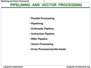
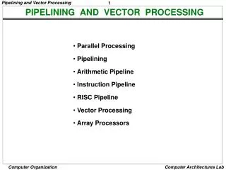
Basic concepts Handling resource conflicts Data hazards Handling branches Performance enhancements Example implementations Pentium PowerPC SPARC MIPS Vector processors Architecture Advantages Cray X-MP Vector length Vector stride Chaining Performance Pipeline Vector processing Outline S. Dandamudi
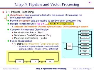
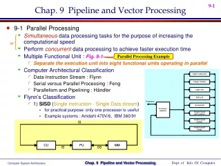
Basic Concepts • Pipelining allows overlapped execution to improve throughput • Introduction given in Chapter 1 • Pipelining can be applied to various functions • Instruction pipeline • Five stages • Fetch, decode, operand fetch, execute, write-back • FP add pipeline • Unpack: into three fields • Align: binary point • Add: aligned mantissas • Normalize: pack three fields after normalization S. Dandamudi
Basic Concepts (cont’d) S. Dandamudi
Basic Concepts (cont’d) Serial execution: 20 cycles Pipelined execution: 8 cycles S. Dandamudi
Basic Concepts (cont’d) • Pipelining requires buffers • Each buffer holds a single value • Uses just-in-time principle • Any delay in one stage affects the entire pipeline flow • Ideal scenario: equal work for each stage • Sometimes it is not possible • Slowest stage determines the flow rate in the entire pipeline S. Dandamudi
Basic Concepts (cont’d) • Some reasons for unequal work stages • A complex step cannot be subdivided conveniently • An operation takes variable amount of time to execute • EX: Operand fetch time depends on where the operands are located • Registers • Cache • Memory • Complexity of operation depends on the type of operation • Add: may take one cycle • Multiply: may take several cycles S. Dandamudi
Basic Concepts (cont’d) • Operand fetch of I2 takes three cycles • Pipeline stalls for two cycles • Caused by hazards • Pipeline stalls reduce overall throughput S. Dandamudi
Basic Concepts (cont’d) • Three types of hazards • Resource hazards • Occurs when two or more instructions use the same resource • Also called structural hazards • Data hazards • Caused by data dependencies between instructions • Example: Result produced by I1 is read by I2 • Control hazards • Default: sequential execution suits pipelining • Altering control flow (e.g., branching) causes problems • Introduce control dependencies S. Dandamudi
Handling Resource Conflicts • Example • Conflict for memory in clock cycle 3 • I1 fetches operand • I3 delays its instruction fetch from the same memory S. Dandamudi
Handling Resource Conflicts (cont’d) • Minimizing the impact of resource conflicts • Increase available resources • Prefetch • Relaxes just-in-time principle • Example: Instruction queue S. Dandamudi
Data Hazards • Example I1: add R2,R3,R4 /* R2 = R3 + R4 */ I2: sub R5,R6,R2 /* R5 = R6 – R2 */ • Introduces data dependency between I1 and I2 S. Dandamudi
Data Hazards (cont’d) • Three types of data dependencies require attention • Read-After-Write (RAW) • One instruction writes that is later read by the other instruction • Write-After-Read (WAR) • One instruction reads from register/memory that is later written by the other instruction • Write-After-Write (WAW) • One instruction writes into register/memory that is later written by the other instruction • Read-After-Read (RAR) • No conflict S. Dandamudi
Data Hazards (cont’d) • Data dependencies have two implications • Correctness issue • Detect dependency and stall • We have to stall the SUB instruction • Efficiency issue • Try to minimize pipeline stalls • Two techniques to handle data dependencies • Register interlocking • Also called bypassing • Register forwarding • General technique S. Dandamudi
Data Hazards (cont’d) • Register interlocking • Provide output result as soon as possible • An Example • Forward 1 scheme • Output of I1 is given to I2 as we write the result into destination register of I1 • Reduces pipeline stall by one cycle • Forward 2 scheme • Output of I1 is given to I2 during the IE stage of I1 • Reduces pipeline stall by two cycles S. Dandamudi
Data Hazards (cont’d) S. Dandamudi
Data Hazards (cont’d) • Implementation of forwarding in hardware • Forward 1 scheme • Result is given as input from the bus • Not from A • Forward 2 scheme • Result is given as input from the ALU output S. Dandamudi
Data Hazards (cont’d) • Register interlocking • Associate a bit with each register • Indicates whether the contents are correct • 0 : contents can be used • 1 : do not use contents • Instructions lock the register when using • Example • Intel Itanium uses a similar bit • Called NaT (Not-a-Thing) • Uses this bit to support speculative execution • Discussed in Chapter 14 S. Dandamudi
Data Hazards (cont’d) • Example I1: add R2,R3,R4 /* R2 = R3 + R4 */ I2: sub R5,R6,R2 /* R5 = R6 – R2 */ • I1 locks R2 for clock cycles 3, 4, 5 S. Dandamudi
Data Hazards (cont’d) • Register forwarding vs. Interlocking • Forwarding works only when the required values are in the pipeline • Intrerlocking can handle data dependencies of a general nature • Example load R3,count ; R3 = count add R1,R2,R3 ; R1 = R2 + R3 • add cannot use R3 value until load has placed the count • Register forwarding is not useful in this scenario S. Dandamudi
Handling Branches • Braches alter control flow • Require special attention in pipelining • Need to throw away some instructions in the pipeline • Depends on when we know the branch is taken • First example (next slide) • Discards three instructions I2, I3 and I4 • Pipeline wastes three clock cycles • Called branch penalty • Reducing branch penalty • Determine branch decision early • Next example: penalty of one clock cycle S. Dandamudi
Handling Branches (cont’d) S. Dandamudi
Handling Branches (cont’d) • Delayed branch execution • Effectively reduces the branch penalty • We always fetch the instruction following the branch • Why throw it away? • Place a useful instruction to execute • This is called delay slot Delay slot add R2,R3,R4 branch target sub R5,R6,R7 . . . branch target add R2,R3,R4 sub R5,R6,R7 . . . S. Dandamudi
Branch Prediction • Three prediction strategies • Fixed • Prediction is fixed • Example: branch-never-taken • Not proper for loop structures • Static • Strategy depends on the branch type • Conditional branch: always not taken • Loop: always taken • Dynamic • Takes run-time history to make more accurate predictions S. Dandamudi
Branch Prediction (cont’d) • Static prediction • Improves prediction accuracy over Fixed S. Dandamudi
Branch Prediction (cont’d) • Dynamic branch prediction • Uses runtime history • Takes the past n branch executions of the branch type and makes the prediction • Simple strategy • Prediction of the next branch is the majority of the previous n branch executions • Example: n = 3 • If two or more of the last three branches were taken, the prediction is “branch taken” • Depending on the type of mix, we get more than 90% prediction accuracy S. Dandamudi
Branch Prediction (cont’d) • Impact of past n branches on prediction accuracy S. Dandamudi
Branch Prediction (cont’d) S. Dandamudi
Branch Prediction (cont’d) S. Dandamudi
Performance Enhancements • Several techniques to improve performance of a pipelined system • Superscalar • Replicates the pipeline hardware • Superpipelined • Increases the pipeline depth • Very long instruction word (VLIW) • Encodes multiple operations into a long instruction word • Hardware schedules these instructions on multiple functional units • No run-time analysis S. Dandamudi
Performance Enhancements • Superscalar • Dual pipeline design • Instruction fetch unit gets two instructions per cycle S. Dandamudi
Performance Enhancements (cont’d) • Dual pipeline design assumes that instruction execution takes the same time • In practice, instruction execution takes variable amount of time • Depends on the instruction • Provide multiple execution units • Linked to a single pipeline • Example (next slide) • Two integer units • Two FP units • These designs are called superscalar designs S. Dandamudi
Performance Enhancements (cont’d) S. Dandamudi
Performance Enhancements (cont’d) • Superpipelined processors • Increases pipeline depth • Ex: Divide each processor cycle into two or more subcycles • Example: MIPS R40000 • Eight-stage instruction pipeline • Each stage takes half the master clock cycle IF1 & IF2: instruction fetch, first half & second half RF : decode/fetch operands EX : execute DF1 & DF2: data fetch (load/store): first half and second half TC : load/store check WB : write back S. Dandamudi
Performance Enhancements (cont’d) S. Dandamudi
Performance Enhancements (cont’d) • Very long instruction word (VLIW) • With multiple resources, instruction scheduling is important to keep these units busy • In most processors, instruction scheduling is done at run-time by looking at instructions in the instructions queue • VLIW architectures move the job of instruction scheduling from run-time to compile-time • Implies moving from hardware to software • Implies moving from online to offline analysis • More complex analysis can be done • Results in simpler hardware S. Dandamudi
Performance Enhancements (cont’d) • Out-of-order execution add R1,R2,R3 ;R1 = R2 + R3 sub R5,R6,R7 ;R5 = R6 – R7 and R4,R1,R5 ;R4 = R1 AND R5 xor R9,R9,R9 ;R9 = R9 XOR R9 • Out-of-order execution allows executing XOR before AND • Cycle 1: add, sub, xor • Cycle 2: and • More on this in Chapter 14 S. Dandamudi
Performance Enhancements (cont’d) • Each VLIW instruction consists of several primitive operations that can be executed in parallel • Each word can be tens of bytes wide • Multiflow TRACE system: • Uses 256-bit instruction words • Packs 7 different operations • A more powerful TRACE system • Uses 1024-bit instruction words • Packs as many as 28 operations • Itanium uses 128-bit instruction bundles • Each consists of three 41-bit instructions S. Dandamudi
Example Implementations • We look at instruction pipeline details of four processors • Cover both RISC and CISC • CISC • Pentium • RISC • PowerPC • SPARC • MIPS S. Dandamudi
Pentium Pipeline • Pentium • Uses dual pipeline design to achieve superscalar execution • U-pipe • Main pipeline • Can execute any Pentium instruction • V-pipe • Can execute only simple instructions • Floating-point pipeline • Uses the dynamic branch prediction strategy S. Dandamudi
Pentium Pipeline (cont’d) S. Dandamudi
Pentium Pipeline (cont’d) • Algorithm used to schedule the U- and V-pipes • Decode two consecutive instructions I1 and I2 IF (I1 and I2 are simple instructions) AND (I1 is not a branch instruction) AND (destination of I1 source of I2) AND (destination of I1 destination of I2) THEN Issue I1 to U-pipe and I2 to V-pipe ELSE Issue I1 to U-pipe S. Dandamudi
Pentium Pipeline (cont’d) • Integer pipeline • 5-stages • FP pipeline • 8-stages • First 3 stages are common S. Dandamudi
Pentium Pipeline (cont’d) • Integer pipeline • Prefetch (PF) • Prefetches instructions and stores in the instruction buffer • First decode (D1) • Decodes instructions and generates • Single control word (for simple operations) • Can be executed directly • Sequence of control words (for complex operations) • Generated by a microprogrammed control unit • Second decode (D2) • Control words generated in D1 are decoded • Generates necessary operand addresses S. Dandamudi
Pentium Pipeline (cont’d) • Execute (E) • Depends on the type of instruction • Accesses either operands from the data cache, or • Executes instructions in the ALU or other functional units • For register operands • Operation is performed during E stage and results are written back to registers • For memory operands • D2 calculates the operand address • E stage fetches the operands • Another E stage is added to execute in case of cache hit • Write back (WB) • Writes the result back S. Dandamudi
Pentium Pipeline (cont’d) • 8-stage FP Pipeline • First three stages are the same as in the integer pipeline • Operand fetch (OF) • Fetches necessary operands from data cache and FP registers • First execute (X1) • Initial operation is done • If data fetched from cache, they are written to FP registers S. Dandamudi
Pentium Pipeline (cont’d) • Second execute (X2) • Continues FP operation initiated in X1 • Write float (WF) • Completes the FP operation • Writes the result to FP register file • Error reporting (ER) • Used for error detection and reporting • Additional processing may be required to complete execution S. Dandamudi
PowerPC Pipeline • PowerPC 604 processor • 32 general-purpose registers (GPRs) • 32 floating-point registers (FPRs) • Three basic execution units • Integer • Floating-point • Load/store • A branch processing unit • A completion unit • Superscalar • Issues up to 4 instructions/clock S. Dandamudi
PowerPC Pipeline (cont’d) S. Dandamudi
PowerPC Pipeline (cont’d) • Integer unit • Two single-cycle units (SCIU) • Execute most integer instructions • Take only one cycle to execute • One multicycle unit (MCIU) • Executes multiplication and division • Multiplication of two 32-bit integers takes 4 cycles • Division takes 20 cycles • Floating-point unit (FPU) • Handles both single- and double precision FP operations S. Dandamudi