Download
1 / 34
370 likes | 576 Views
Lecture 11: Scale Free Networks. CS 765 Complex Networks. Slides are modified from Networks: Theory and Application by Lada Adamic. Scale-free networks. Many real world networks contain hubs: highly connected nodes Usually the distribution of edges is extremely skewed.

E N D
Lecture 11:Scale Free Networks CS 765 Complex Networks Slides are modified from Networks: Theory and Application by Lada Adamic
Scale-free networks • Many real world networks contain hubs: highly connected nodes • Usually the distribution of edges is extremely skewed many nodes with few edges number of nodes with so many edges fat tail: a few nodes with a very large numberof edges number of edges no “typical” number of edges
But is it really a power-law? • A power-law will appear as a straight line on a log-log plot: • A deviation from a straight line could indicate a different distribution: • exponential • lognormal log(# nodes) log(# edges)
Scale-free networks http://ccl.northwestern.edu/netlogo/models/PreferentialAttachment
What is a heavy tailed-distribution? • Right skew • normal distribution (not heavy tailed) • e.g. heights of human males: centered around 180cm (5’11’’) • Zipf’s or power-law distribution (heavy tailed) • e.g. city population sizes: NYC 8 million, but many, many small towns • High ratio of max to min • human heights • tallest man: 272cm (8’11”), shortest man: (1’10”) ratio: 4.8from the Guinness Book of world records • city sizes • NYC: pop. 8 million, Duffield, Virginia pop. 52, ratio: 150,000
Normal (also called Gaussian) distribution of human heights average value close to most typical distribution close to symmetric around average value
Power-law distribution • linear scale • log-log scale • high skew (asymmetry) • straight line on a log-log plot
Power laws are seemingly everywherenote: these are cumulative distributions, more about this in a bit… AOL users visiting sites ‘97 scientific papers 1981-1997 Moby Dick Source: MEJ Newman, ’Power laws, Pareto distributions and Zipf’s law’ bestsellers 1895-1965 AT&T customers on 1 day California 1910-1992
Yet more power laws wars (1816-1980) Moon Solar flares richest individuals 2003 US family names 1990 US cities 2003
Power law distribution • Straight line on a log-log plot • Exponentiate both sides to get that p(x), theprobability of observing an item of size ‘x’ is given by normalizationconstant (probabilities over all x must sum to 1) power law exponent a
1 2 3 10 20 30 100 200 Logarithmic axes • powers of a number will be uniformly spaced • 20=1, 21=2, 22=4, 23=8, 24=16, 25=32, 26=64,….
Fitting power-law distributions • Most common and not very accurate method: • Bin the different values of x and create a frequency histogram ln(x) is the natural logarithm of x, but any other base of the logarithm will give the same exponent of a because log10(x) = ln(x)/ln(10) ln(# of timesx occurred) ln(x) x can represent various quantities, the indegree of a node, the magnitude of an earthquake, the frequency of a word in text
Example on an artificially generated data set • Take 1 million random numbers from a distribution with a = 2.5 • Can be generated using the so-called‘transformation method’ • Generate random numbers r on the unit interval0≤r<1 • then x = (1-r)-1/(a-1) is a random power law distributed real number in the range 1 ≤ x <
Linear scale plot of straight bin of the data • Power-law relationship not as apparent • Only makes sense to look at smallest bins whole range first few bins
Log-log scale plot of straight binning of the data • Same bins, but plotted on a log-log scale here we have tens of thousands of observations when x < 10 Noise in the tail: Here we have 0, 1 or 2 observations of values of x when x > 500 Actually don’t see all the zero values because log(0) =
Log-log scale plot of straight binning of the data • Fitting a straight line to it via least squares regression will give values of the exponent a that are too low fitted a true a
have few bins here have many more bins here What goes wrong with straightforward binning • Noise in the tail skews the regression result
First solution: logarithmic binning • bin data into exponentially wider bins: • 1, 2, 4, 8, 16, 32, … • normalize by the width of the bin evenly spaced datapoints less noise in the tail of the distribution • disadvantage: binning smoothes out data but also loses information
Second solution: cumulative binning • No loss of information • No need to bin, has value at each observed value of x • But now have cumulative distribution • i.e. how many of the values of x are at least X • The cumulative probability of a power law probability distribution is also power law but with an exponent a - 1
Fitting via regression to the cumulative distribution • fitted exponent (2.43) much closer to actual (2.5)
Where to start fitting? • some data exhibit a power law only in the tail • after binning or taking the cumulative distribution you can fit to the tail • so need to select an xmin the value of x where you think the power-law starts • certainly xmin needs to be greater than 0, because x-a is infinite at x = 0
Example: • Distribution of citations to papers • power law is evident only in the tail • xmin > 100 citations xmin Source: MEJ Newman, ’Power laws, Pareto distributions and Zipf’s law
Maximum likelihood fitting – best • You have to be sure you have a power-law distribution • this will just give you an exponent but not a goodness of fit • xi are all your datapoints, • there are n of them • for our data set we get a = 2.503 – pretty close!
What does it mean to be scale free? • A power law looks the same no mater what scale we look at it on (2 to 50 or 200 to 5000) • Only true of a power-law distribution! • p(bx) = g(b) p(x) • shape of the distribution is unchanged except for a multiplicative constant • p(bx) = (bx)-a = b-a x-a log(p(x)) x →b*x log(x)
But, not everything is a power law • number of sightings of 591 bird species in the North American Bird survey in 2003. cumulative distribution • another example: • size of wildfires (in acres) Source: MEJ Newman, ’Power laws, Pareto distributions and Zipf’s law’
Not every network is power law distributed • reciprocal, frequent email communication • power grid • Roget’s thesaurus • company directors…
Another common distribution: power-lawwith an exponential cutoff • p(x) ~ x-a e-x/k starts out as a power law ends up as an exponential but could also be a lognormal or double exponential…
Zipf &Pareto: what they have to do with power-laws • George Kingsley Zipf, a Harvard linguistics professor, sought to determine the 'size' of the 3rd or 8th or 100th most common word. • Size here denotes the frequency of use of the word in English text, and not the length of the word itself. • Zipf's law states that the size of the r'th largest occurrence of the event is inversely proportional to its rank: y ~ r -b , with b close to unity.
Zipf &Pareto: what they have to do with power-laws • The Italian economist Vilfredo Pareto was interested in the distribution of income. • Pareto’s law is expressed in terms of the cumulative distribution • the probability that a person earns X or more P[X > x] ~ x-k • Here we recognize k as just a -1, where a is the power-law exponent
So how do we go from Zipf to Pareto? • The phrase "The r th largest city has n inhabitants" is equivalent to saying "r cities have n or more inhabitants". • This is exactly the definition of the Pareto distribution, except the x and y axes are flipped. • for Zipf, r is on the x-axis and n is on the y-axis, • for Pareto, r is on the y-axis and n is on the x-axis. • Simply inverting the axes, • if the rank exponent is b, i.e. n ~ r-bfor Zipf, (n = income, r = rank of person with income n) • then the Pareto exponent is 1/b so that r ~ n-1/b (n = income, r = number of people whose income is n or higher)
Zipf’s Law and city sizes (~1930) source: Luciano Pietronero
80/20 rule (Pareto principle) • Joseph M. Juran observed that 80% of the land in Italy was owned by 20% of the population. • The fraction W of the wealth in the hands of the richest P of the the population is given byW = P(a-2)/(a-1) • Example: US wealth: a = 2.1 • richest 20% of the population holds 86% of the wealth