Download
1 / 61
610 likes | 784 Views
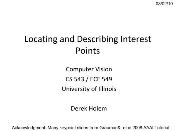
02/07/12. Locating and Describing Interest Points. Computer Vision CS 543 / ECE 549 University of Illinois Derek Hoiem. Acknowledgment: Many keypoint slides from Grauman&Leibe 2008 AAAI Tutorial. This section: correspondence and alignment.

E N D
02/07/12 Locating and Describing Interest Points Computer Vision CS 543 / ECE 549 University of Illinois Derek Hoiem Acknowledgment: Many keypoint slides from Grauman&Leibe 2008 AAAI Tutorial
This section: correspondence and alignment • Correspondence: matching points, patches, edges, or regions across images ≈
This section: correspondence and alignment • Alignment: solving the transformation that makes two things match better T
Example: fitting an 2D shape template A Slide from Silvio Savarese
Example: fitting a 3D object model Slide from Silvio Savarese
Example: estimating “fundamental matrix” that corresponds two views Slide from Silvio Savarese
Example: tracking points x x x frame 22 frame 0 frame 49 Your problem 1 for HW 2!
HW 2 • Interest point detection and tracking • Detect trackable points • Track them across 50 frames • In HW 3, you will use these tracked points for structure from motion frame 49 frame 0 frame 22
HW 2 • Alignment of object edge images • Compute a transformation that aligns two edge maps
HW 2 • Initial steps of object alignment • Derive basic equations for interest-point based alignment
This class: interest points • Note: “interest points” = “keypoints”, also sometimes called “features” • Many applications • tracking: which points are good to track? • recognition: find patches likely to tell us something about object category • 3D reconstruction: find correspondences across different views
Human eye movements Yarbus eye tracking
Human eye movements Se Study by Yarbus Change blindness: http://www.simonslab.com/videos.html
This class: interest points original • Suppose you have to click on some point, go away and come back after I deform the image, and click on the same points again. • Which points would you choose? deformed
Overview of Keypoint Matching 1. Find a set of distinctive key- points 2. Define a region around each keypoint A1 B3 3. Extract and normalize the region content A2 A3 B2 B1 4. Compute a local descriptor from the normalized region 5. Match local descriptors K. Grauman, B. Leibe
Goals for Keypoints Detect points that are repeatable and distinctive
Key trade-offs B3 A1 A2 A3 B2 B1 Detection More Points More Repeatable Robust detection Precise localization Robust to occlusion Works with less texture Description More Flexible More Distinctive Robust to expected variations Maximize correct matches Minimize wrong matches
Choosing interest points Where would you tell your friend to meet you?
Choosing interest points Where would you tell your friend to meet you?
Many Existing Detectors Available Hessian & Harris [Beaudet ‘78], [Harris ‘88] Laplacian, DoG[Lindeberg ‘98], [Lowe 1999] Harris-/Hessian-Laplace[Mikolajczyk & Schmid ‘01] Harris-/Hessian-Affine [Mikolajczyk & Schmid ‘04] EBR and IBR [Tuytelaars & Van Gool ‘04] MSER[Matas ‘02] Salient Regions [Kadir & Brady ‘01] Others… K. Grauman, B. Leibe
Harris Detector [Harris88] • Second moment matrix Intuition: Search for local neighborhoods where the image content has two main directions (eigenvectors). K. Grauman, B. Leibe
Ix Iy Harris Detector [Harris88] • Second moment matrix 1. Image derivatives (optionally, blur first) Iy2 IxIy Ix2 2. Square of derivatives g(IxIy) g(Ix2) g(Iy2) 3. Gaussian filter g(sI) 4. Cornerness function – both eigenvalues are strong 5. Non-maxima suppression har
Harris Detector: Mathematics Want large eigenvalues, and small ratio We know Leads to (k :empirical constant, k = 0.04-0.06) Nice brief derivation on wikipedia
Harris Detector – Responses [Harris88] Effect: A very precise corner detector.
Hessian Detector [Beaudet78] • Hessian determinant Ixx Iyy Ixy Intuition: Search for strongcurvature in two orthogonal directions K. Grauman, B. Leibe
Hessian Detector [Beaudet78] • Hessian determinant Ixx Iyy Ixy In Matlab: K. Grauman, B. Leibe
Hessian Detector – Responses [Beaudet78] Effect: Responses mainly on corners and strongly textured areas.
Automatic Scale Selection How to find corresponding patch sizes? K. Grauman, B. Leibe
Automatic Scale Selection • Function responses for increasing scale (scale signature) K. Grauman, B. Leibe
Automatic Scale Selection • Function responses for increasing scale (scale signature) K. Grauman, B. Leibe
Automatic Scale Selection • Function responses for increasing scale (scale signature) K. Grauman, B. Leibe
Automatic Scale Selection • Function responses for increasing scale (scale signature) K. Grauman, B. Leibe
Automatic Scale Selection • Function responses for increasing scale (scale signature) K. Grauman, B. Leibe
Automatic Scale Selection • Function responses for increasing scale (scale signature) K. Grauman, B. Leibe
What Is A Useful Signature Function? • Difference-of-Gaussian = “blob” detector K. Grauman, B. Leibe
Difference-of-Gaussian (DoG) = - K. Grauman, B. Leibe
DoG – Efficient Computation • Computation in Gaussian scale pyramid Sampling withstep s4=2 s s s s Original image K. Grauman, B. Leibe
Find local maxima in position-scale space of Difference-of-Gaussian s5 s4 s3 s2 List of(x, y, s) s K. Grauman, B. Leibe
Results: Difference-of-Gaussian K. Grauman, B. Leibe
Orientation Normalization p 2 0 • Compute orientation histogram • Select dominant orientation • Normalize: rotate to fixed orientation [Lowe, SIFT, 1999] T. Tuytelaars, B. Leibe
Maximally Stable Extremal Regions [Matas ‘02] • Based on Watershed segmentation algorithm • Select regions that stay stable over a large parameter range K. Grauman, B. Leibe
Example Results: MSER K. Grauman, B. Leibe
Available at a web site near you… • For most local feature detectors, executables are available online: • http://www.robots.ox.ac.uk/~vgg/research/affine • http://www.cs.ubc.ca/~lowe/keypoints/ • http://www.vision.ee.ethz.ch/~surf K. Grauman, B. Leibe
Local Descriptors • The ideal descriptor should be • Robust • Distinctive • Compact • Efficient • Most available descriptors focus on edge/gradient information • Capture texture information • Color rarely used K. Grauman, B. Leibe
Local Descriptors: SIFT Descriptor • Histogram of oriented gradients • Captures important texture information • Robust to small translations / affine deformations [Lowe, ICCV 1999] K. Grauman, B. Leibe
Details of Lowe’s SIFT algorithm • Run DoG detector • Find maxima in location/scale space • Remove edge points • Find all major orientations • Bin orientations into 36 bin histogram • Weight by gradient magnitude • Weight by distance to center (Gaussian-weighted mean) • Return orientations within 0.8 of peak • Use parabola for better orientation fit • For each (x,y,scale,orientation), create descriptor: • Sample 16x16 gradient mag. and rel. orientation • Bin 4x4 samples into 4x4 histograms • Threshold values to max of 0.2, divide by L2 norm • Final descriptor: 4x4x8 normalized histograms Lowe IJCV 2004
Matching SIFT Descriptors • Nearest neighbor (Euclidean distance) • Threshold ratio of nearest to 2nd nearest descriptor Lowe IJCV 2004